Some mathematic derivation in the blog is based on the fundation of calculus and linear algebra which can be found in the below linked
1. Recurrent Neural Networks
Examples of sequence data:
- Speech Recognition: given audio clip X —-> text Y (both input and output sequence data)
- music generation: output is sequence(音乐), input maybe music genre you want to generate or nothing
- sentiment classfication: Movie: “there is nothing to like in this move” —> positive / negative, score from 1 to 5
- DNA sequence Analysis: given DNA AGCCTGA… —> label which part of DNA sequence corresponds to a protein
- machine translation: sentences -> sentences in a different language
- video activty recogntion : a sequence of video => recognize the activity
- Name entity recognation:sentence –> ask the people in the sentence
- sometimes X and Y can be different lengths
- sometimes X和Y(example 4,7)是同样长度的
- sometimes only either X or Y is sequence的 (example 2)
Notation
Motivating Example: Named Entity Recognition(used by search engines to index all of last 24 hours news of all people/ companies/ name/ times/ llocations / countries names etcs mentioned in the news articles so that they can index them appropriately)
Below example for Named Entity Recognition not perfect representation, some sophisticated output representations tell the start and ends of people’s names in the sentence
x: Harry Potter and Hermione Granger invented a new spell
y   1     1     0     1        1       0      0  0   0
- \(x^{({i})<{t}>}\): t-th element of the sequence in ith- training example. Different training examples in training set can have different length. In above example,\(x^{({i})<{1}>}\) represent Harry
- \(y^{({i})<{t}>}\): t-th element in the output sequence of ith training example
- \(T_x^{i}\): length of input sequnece in i-th traning example, in above example,\(T_x^{i} = 9\)
- \(T_y^{i}\): length of output sequence in i-th training example .in above example,\(T_y^{i} = 9\), Note ,\(T_x^{i}\) and \(T_y^{i}\) can be different
representing words: :use Vocabulary(dictionary) and give each word an index,
e.g. size 10000 (Quite small for modern NLP applications. For commercial applications, vocabulary size is 30,000 - 50,000. Some large internet companies use 1 million vocabulary size )
- Look at training set and find top 10,000 occurring words
- Or look at some online dictionary to tell you what are the most common 10,000 words in English Language
- Use One hot representation(only 一个one and zero everywhere else) to represent each of these words
- if encounter word not in vocabulary,create a new token or a new fake word called unknown word
<unk>
Recurrent Neural Network Model:
Why not a standard network?(e.g. sentiment in NLP ) problems:
- Input, output can be different lengths in different example (不是所有的input的都是一样长度)
- Maybe for every sentence has a maximum length. can pad or zero-pad every inputs up to maximum length. But it still not a good representation
- Doesn’t share features learned across different positions of text
- Maybe Harry on position one gives a sign(implies) that position t would be a person’s name
- Parameter size is large, e.g. use 10,000 one hot vector size and 9 sequence of input, input shape is
9 x 10000, weight matrix will end up enormous number of parameters
RNN doesn’t have above disadvantages
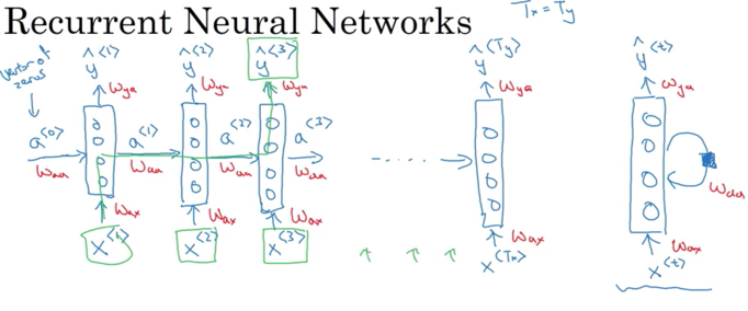
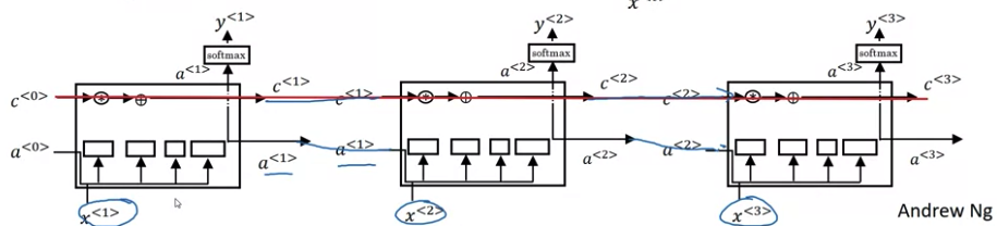
Below architecture for \(T_x = T_y\). Each timestep, recurrent neural network pass activation to next time step. To kick off the whole thing, make-up activation of \(a^{<0>}\)(usually vector of zeros most common , and some researchers initialize it randomly) at time zero
- Read first word \(x^{<1>}\), take this word and feed into a neural network layer and predict a output \(\hat y^{<1>}\)
- Read the second word \(x^{<2>}\), instead of just predicting \(\hat y_2\) using only \(x^{<2>}\), also gets some information from step one. The activation value from step one passed to step two.
- To output \(\hat y^{<3>}\), RNN input the third word \(x^{<3>}\) and activation \(a^{<2>}\) from step two
下图左面是unroll diagram, 右侧一个单独的是 rolled diagram
Recurrent Neural Network scans through the data from left to right. The parameters it uses for each time step are shared.
- The same \(W_{ax}\) used for every time step. \(W_{ax}\), govern the connection between \(x_{<i+1>}\) to hidden layer
- \(W_{aa}\), (from activation to activation) govern the horizontal activation connection. It is the same \(W_{aa}\) for every timestep
- \(W_{ya}\) (from activition to y) (用x得到y like quantity) governs the output prediction
So when make prediction for \(y_3\), gets the information not only from \(x_3\) but also the information from \(x_1\) and \(x_2\)
One weakness for this RNN: only use information that is earlier in the sequence but not information later in the sequence to make a prediction (Bidirection RNN (BRNN) can solve this problem)e.g. when prediciting \(y_{<3>}\) not use \(x_{<4>}\)
- e.g. He said “Teddy Roosevelt was a great President and He said “Teddy bears are on sale”. Given only first three words, it is not possible to know if Teddy is part of a person’s name. In order to decide whether Teddy is part of person’s name. It’s really useful to know not just information from first two words but also latter words
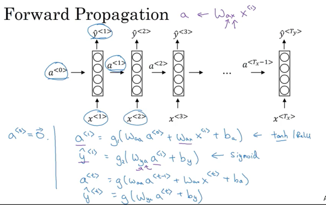
Forward Propagation
\[\begin{align} a^{<{0}>} &= \vec0 \\ a^{<{1}>} &= g_1\left(W_{aa}\cdot a^{<{0}>}+ W_{ax}\cdot X^{<{1}>} + b_a \right) -> \bbox[yellow]{\text{ often tanh(more common)/ReLu function}} \\ y^{<{1}>} &= g_2\left(W_{ya}\cdot a^{<{1}>} + b_y \right) -> \bbox[yellow]{\text{ often sigmoid/softmax function}} \end{align}\]More general representation
\[\begin{align} a^{<{t}>} &= g\left(W_{aa}\cdot a^{<{t-1}>}+ W_{ax}\cdot X^{<{t}>} + b_a \right) -> \bbox[yellow]{\text{ often tanh(more common)/ReLu function}} \\ y^{<{t}>} &= g\left(W_{ya}\cdot a^{<{t}>} + b_y \right) -> \bbox[yellow]{\text{ often sigmoid/softmax function}} \end{align}\]For output activation function, if it is binary classification problem, use sigmoid. If it is k-classification problem, use softmax
Simplified Notation:
\[a^{<{t}>} = g\left(W_{a} \left[ a^{<{t-1}>}, x^{<{t}>} \right] + b_a \right)\] \[y^{<{t}>} = g\left(W_y\cdot a^{<{t}>} + b_y \right)\]Where \(W_a, b_a\) denotes to compute activation and \(W_y, b_y\) denote to compute to y-like quantity
\[W_{a} = \left[ W_{aa} \mid W_{ax} \right]\] \[\left[ a^{<{t-1}>}, x^{<{t}>} \right] = \begin{bmatrix} a^{<{t-1}>} \\[2ex] \hline \\ x^{<{t}>} \end{bmatrix}\] \[\left[ W_{aa} \mid W_{ax} \right] \begin{bmatrix} a^{<{t-1}>} \\[2ex] \hline \\ x^{<{t}>} \end{bmatrix} = W_{aa}\cdot a^{<{t-1}>}+ W_{ax}\cdot X^{<{t}>}\]e.g. if \(a^{<{t}>}\) is 100 x 1, \(x^{<{t}>}\) is 10000 x 1, \(W_{aa}\) is 100 x 100 and \(W_{ax}\) is 100 x 10000 matrix. So stacking \(W_{aa}, W_{ax}\) together,
Backpropagation
Backpropagation through time: For fowardprop scans from left to right and increase the indices time t, whereas for back propagation go from right to left
Single Loss Function( Cross Entropy Loss) associated with a single prediction for single position or single time set:
\[L^{<{t}>}\left( \hat y^{<{t}>}, y^{<{t}>} \right) = - y^{<{t}>}log \left( \hat y^{<{t}>} \right) - \left( 1- y^{<{t}>} \right) log\left(1- \hat y^{<{t}>} \right)\]Overall Loss Function: sume up all loss for all timestamps
\[L \left( \hat y , y \right) = \displaystyle \sum_{t=1}^{T_x} {L^{<{t}>} \left( \hat y^{<{t}>}, y^{<{t}>} \right) }\]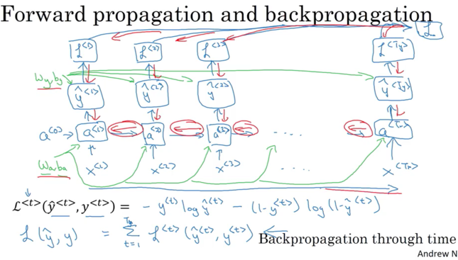
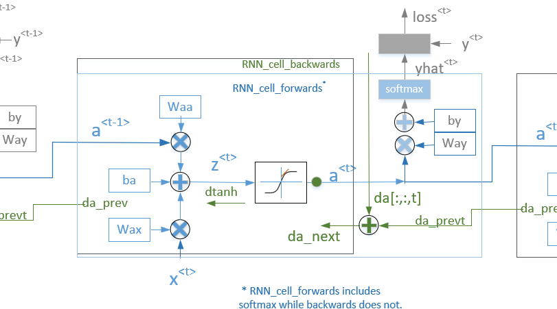
* denote element-wise product, derivate with respect to activation
derivate with respect to loss
\[\begin{align} \frac{\partial L }{\partial W_{ax}} = \frac{\partial L }{\partial a^{<{t}>}}\frac{\partial a^{<{t}>} }{\partial W_{ax}} &= \left(d_a^{<{t}>}*\left(1- tanh \left(W_{aa} a^{<{t-1}>} + W_{ax} x^{<{t}>} + b\right)^2 \right)\right) \left(x^{<{t}>}\right)^T \\ \frac{\partial L }{\partial W_{aa}} = \frac{\partial L }{\partial a^{<{t}>}}\frac{\partial a^{<{t}>} }{\partial W_{aa}} &= \left( d_a^{<{t}>}* \left(1- tanh \left(W_{aa} a^{<{t-1}>} + W_{ax} x^{<{t}>} + b \right)^2 \right)\right) \left(a^{<{t-1}>}\right)^T \\ \frac{\partial L }{\partial b} = \frac{\partial L }{\partial a^{<{t}>}}\frac{\partial a^{<{t}>} }{\partial b} &= \sum_{batch} \left( d_a^{<{t}>}* \left(1- tanh \left(W_{aa} a^{<{t-1}>} + W_{ax} x^{<{t}>} + b \right)^2 \right) \right) \\ \frac{\partial L }{\partial x^{<{t}>}} = \frac{\partial L }{\partial a^{<{t}>}}\frac{\partial a^{<{t}>} }{\partial x^{<{t}>}} &= W_{ax}^T \left(d_a^{<{t}>}* \left(1- tanh \left(W_{aa} a^{<{t-1}>} + W_{ax} x^{<{t}>} + b \right)^2 \right)\right) \\ \frac{\partial L }{\partial a^{<{t-1}>}} = \frac{\partial L }{\partial a^{<{t}>}}\frac{\partial a^{<{t}>} }{\partial a^{<{t-1}>}} &= W_{aa}^T \left( d_a^{<{t}>}* \left(1- tanh \left(W_{aa} a^{<{t-1}>} + W_{ax} x^{<{t}>} + b \right)^2 \right) \right) \\ \text{where, } d_a^{<{t}>} &= \frac{\partial L }{\partial a^{<{t}>}} = \left(\underbrace{\frac{\partial L }{\partial z}}_{\text{softmax/sigmoid derivative}} \frac{\partial z^{<{t}>}}{\partial a^{<{t}>}} + d_a^{<{t+1}>} \right) \\ & = \left(W_{ya}^T \frac{\partial L }{\partial z} + d_a^{<{t+1}>} \right) \\ \end{align}\]For \(d a^{<{t}>}\), When \(a^{<{t}>}\) changes, it affects the cost function in 2 ways. First, it changes the output of the layer t (the value of \(y^{<{t}>}\)) and second, it changes all further cells / output values to the right (t+1, t+2 ….).
So, the derivative of cost function by \(a^{<{t}>}\) is a sum of two items: partial derivative of cost by \(y^{<{t}>}\) (that’s the function argument da[:,:,t] in the below diagram), and sum of derivatives of all further laters (that’s the da_prevt from the cell to the right). BTW, as expected \(d a^{<{t}>}\) is zero for the last cell.
More Detailed Derivation More Detailed Derivation2
RNN Architectures
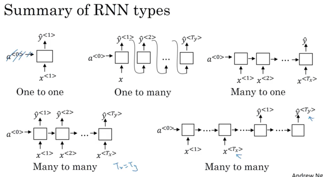
- Many to Many Architectures: 比如named entity recognition,输入的每word,都有输出0,1(表示是不是人名); 注:many-to-many, input length 和 Output length可以相同,也可以不同,比如翻译先把法语(encoder)句子读完,然后一个一个generate 英语(decoder), English and French sentences can be different length(图片的右下方)
- Many to One Architectures: Sentiment Classification: X is sequence(review),y might be 0 and 1 (positive review/negative review), or 1 to 5 (one star? two star?five-star review)
- One to One Architectures: standard neural network
- One to Many Architectures: X could be genre of music or what is the first note of the music you want or x 可以是null. e.g. music generation output a set of notes (\(y^{<{1}>}, y^{<{2}>}, ..., y^{<{T_y}>}\)) 代表a piece of music
Language Model
Speech recognition
The apple and pair salad vs The apple and pear salad
第二个更likely. That is a good speech recognition system would output even though these two sentences sound exactly the same. The way speech recognition system picks the second is by using a lanuage model that tells the probability of either of those two sentences.
P(The apple and pair salad) = \(3.2\times10^{-13}\)
P(The apple and pair salad) = \(5.7\times10^{-10}\)
Language model tell you the probability of a sentence: P(sentence) = ?. It is the fundamental component in Speech Recognition systems and Machine Translation systems, where translation systems want output only sentences that are likely. Estimate the probabilities ofp articular sequence of words
How to build a lanuage model?
- Need a training set comprising large corpus of English text; corpus: NLP terminalogy means a large body/set.
- Tokenize each sentence to form a vocabulary.
- Map each word to one hot vector
- Add extra token
EOS(end of sentences) which can help figure out when a sentence ends。 也可以决定是否把标点符号也tokenize. - 如果word 不在字典中,用
UNKsubstitue for unknown word
- Set \(x^{<t>} = y^{<t-1>}\) for training
RNN Model: each step in the RNN will look at some set of preceding words
- At time 0, \(x^{<1>} = \vec 0\), set \(x_1\) to be all zeros. Also set \(a^{<0>} = \vec 0\)
- \(a^{<1>}\) make a softmax to predict the probability of any word in the dictionary to be the first word \(y^{<1>}\)(What is the chance the first word “Aaron”? what is the chance the first word “cat”? … what is the chance the first word “Zulu”? what is the chance the first word “UNK”?). If vocabulary size is 10002(+
UNKandEOS), there are 10002 softmax outputs
- \(a^{<1>}\) make a softmax to predict the probability of any word in the dictionary to be the first word \(y^{<1>}\)(What is the chance the first word “Aaron”? what is the chance the first word “cat”? … what is the chance the first word “Zulu”? what is the chance the first word “UNK”?). If vocabulary size is 10002(+
- Next step, the job is to try to figure out the second word. Also give the correct first word \(x^{<2>} = y^{<1>}\).
P(average | Cats) - At 3rd step, predict third word, we can give the first two words, \(x^{<3>} = y^{<2>}\). To figure out
P(__ | Cats average)given first two words are cats average
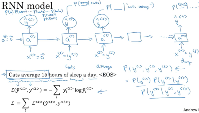
cost function is softmax loss function;
\[L\left( \hat y^{<t>}, y^{<t>} \right) = - \sum_{i} {y_i^{<t>} log \hat y_i^{<t>} }\]Overall loss is just the sume overall time steps of the loss associated with individual predictions
\[L = \sum_{t} {L^{<t>} \left( \hat y^{<t>}, y^{<t>} \right)}\]given the sentence which comprise just three words, the probability of entire sentences will be
\[P\left( y^{<{1}>}, y^{<{2}>}, y^{<{3}>} \right) = P\left( y^{<{1}>}\right) \cdot P\left(y^{<{2}>} \mid y^{<{1}>} \right)\cdot P\left(y^{<{3}>} \mid y^{<{1}>}, y^{<{2}>} \right)\]Sampling Novel Sequence
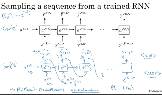
- When at training, pass ground truth \(y^{<{t-1}>}\) as the input for \(x^{<{t}>}\)
- When finish training, pass random sampled \(\hat y^{<{t-1}>}\) from last time step as the input for \(x^{<{t}>}\) (not pick the highest probablity, use the one from random sample)
- Note: for encoder-decoder network to generate translation, need to pick the highest probability using beam search
Sample from distribution to generate noble sequences of words
- At time 0, After get \(\hat y^{<{1}>} (size `10002 x 1`)\),have some softmax probabilities over possible output. random sample according to softmax distribution. The softmax distribution gives what is the chance of first word being Aaron, cats, Zulu.
np.random.choiceto sample according to this distribution defined by output vector proabilities from softmax- 有时可能生成unknown word token, 可以确保algorithm 生成sample 不是unknown token,遇到unknown token, reject and keep sampling until get non-unknown word. Or you can leave it(
UNK) in output if don’t care unknown
- 有时可能生成unknown word token, 可以确保algorithm 生成sample 不是unknown token,遇到unknown token, reject and keep sampling until get non-unknown word. Or you can leave it(
- Next timestamp, expecting \(y^{<{1}>}\) is the input. Take the \(\hat y^{<{1}>}\) you just sample in step 1 (not the correct one) to pass as input. Then softmax will make predict \(\hat y^{<{2}>}\);
- E.g. For sample at timestamp 0, get the first word “The”. Pass “The” as \(x^{<{2}>}\) ,And get softmax distribution
P( _ | the), and sample \(\hat y^{<{2}>}\). 把sample的 pass 到next time step.
- E.g. For sample at timestamp 0, get the first word “The”. Pass “The” as \(x^{<{2}>}\) ,And get softmax distribution
- When to end:
- keep sampling until generate EOS token. , which tells you it the end of a sentence
- 如果没有设置
EOS. then decide to sample 20 个或者100个words 直到到达这个次数(20 or 100 words)
- 如果没有设置
字典除了是vocabulary,也可以是character base, vocabulary = [a,b,c, ... , z, ., ; ,0,1,2,...,9, A,...,Z], lowercases, punctuations, digits, uppercases. Or look at training corpus and look at the chracters that appears there and use that to define the vocabulary
如果想build character level 而不是word level 的,\(y^{<{1}>}, y^{<{2}>}, y^{<{3}>}\)是individual characters instead of individual words,
- E.g. Cat average. \(y^{<1>} = c\), \(y^{<2>} = a\) , \(y^{<3>} = t\), \(y^{<4>} = \text{\space}\)
Advantage: character level don’t worry abut unknown word tokens. Character level is able to assign 比如 Mau(人名/地名), a non-zero probability, whereas if Mau not in vocabulary for word level lanuage model, assign unknown word token
Disadvantage:
- end up much longer sequence. 一句话可能有10个词,但会有很多的characters,
- Character level 不如word level capture long range dependencies between how the earlier parts of sentence aslo affect the later part of the sentence.
- Character level more computationally expensive to train. In NLP, word level language model are still used. But as computers get faster, more and more applications start to look at character level models which are much harder and computationally expensive to train (not widespread today for character level except for specialized applications where need to deal with unknown words or used in more specialized application where have a more specialized vocabulary )
Vanishing gradients
RNN processing data over 1000 or 10000 time steps, that basically a 1000 layer or 10000 layer neural network. So it runs into gradient vanishing or gradient exploding problems
One of the problems with A basic RNN algorithm is that it runs into vanishing gradient problems.
languages that comes earlier 可以影响 later的, e.g. choose was or were
- The cat which …. was full
- The cats which …. were full
The basic RNN not very good at capturing very long-term dependency. because for very deep neural network e.g. 100 layers, the gradient from output y had hard time propagating back to affect the weights of these earlier layers. The outputs of errors associated at latter timestep is difficult to affect computation eariler in the sequence
- 上面的例子, it might be difficult to get a neural network to realize that it needs to memorize if see a singular noun or pural noun to generate “was” or “were”
- Because of the problem, the basic RNN model has many local influences, meaning that output \(\hat y\) is mainly influenced by values close to \(\hat y\)
Exploding Gradient: aslo happen for RNN. When doing backprop, the gradient(slop) not decrease exponentially, instead increase exponentially with the number of layers go through. Whereas Vanish Gradient tends to a bigger problem for RNN
- Can cause parameters become so large and make neural network messed up.
- It is easy to saw and often see NaNs, meaning results of a numerical overflow in neural network computation,
- exploding gradient 可以用gradient clipping,当超过某个threshold得时候,rescale gradient vector so that is not too big. there are clips 不超过最大值, 比如gradient超过\(\left[-10,10\right]\), 就让gradient 保持10 or -10
GRU && LSTM
GRU: Gated Recurrent Unit, capture long range connection and solve Vanishing Gradient Problem.
- There are many different possible versions of how to desgin these units to try to have longer range connections, to have longer range effects, and aggress vandishing gradient problem. GRU is one of the most commonly used versions that researchers found robust and useful for many different problems
c: memory cell. Used to provide a bit of memory to remember e.g. whether cat was singular or puralaoutput activation value, GRU Unit \(c^{<t>} = a^{<t>}\) (LSTM they are different value)- At each time step, produce memory cell \(\tilde c^{<{t}>}\) (the candidate for replacing \(c^{<{t}>}\))
- \(\Gamma_u\): update gate, value between 0 and 1. The update gate will decide whether or not to update \(c^{<{t}>}\) using \(\tilde c^{<{t}>}\). to compute \(\Gamma_u\) use a sigmoid function.
- For most of possible range of input, the value of sigmoid function output will very close to 0 or very close to 1. For intuition, can think of gamma as being either 0 or 1 most of the time.
- 如果gate \(\Gamma_u=1\), set \(c^{<{t}>}\) equal to candidate value \(\tilde c^{<{t}>}\), 比如下面例子, 遇到”cat” gate = 1更新 \(c^{<{t}>}\)为1表示单数, the cat, which already ate…. was full, 从 “cat“ 到 ”was“, gate =0
- Because \(\Gamma_u\) is quite easy set to zero when \(W_u \left[ c^{<{t-1}>}, x^{<{t}>} \right] + b_u\) is large negative value, it is good at maintaining the value of the cell \(c^{<{t}>} = c^{<{t-1}>}\). it won’t suffer that vanish gradient problem , allow nerual network to learn long range dependency
- \(\Gamma_r\): tell how relevant \(c^{<{t-1}>}\) to compute the next candidate \(\tilde c^{<{t}>}\)
GRU Step:
- Takes \(c^{<{t-1}>}\)(= \(a^{<{t}>}\) in GRU) as input also take input \(x^{<{t}>}\).
- Then \(c^{<{t-1}>}\) and \(x^{<{t}>}\) with a set of parameters and through a sigmoid activation function to get relevant gate \(\mathbf{ \Gamma_r }\).
- Then \(c^{<{t-1}>}\) and \(x^{<{t}>}\) combine together with tanh gives \(\mathbf{\tilde c^{<{t}>} }\) (candidate for replacing \(c^{<{t}>}\))
- Then \(c^{<{t-1}>}\) and \(x^{<{t}>}\) with different set of parameters and through a sigmoid activation function to get update gate \(\mathbf{\Gamma_u }\).
- Then take \(c^{<{t-1}>}\)), \(\tilde c^{<{t}>}\) and \(\Gamma_r\) to generate new value for the memory cell \(\mathbf{c^{<{t}>} = a^{<{t}>}}\)
- Also can take \(c^{<{t-1}>}\), \(\tilde c^{<{t}>}\) and \(\Gamma_u\) to pass to a softmax to make a prediction \(\mathbf{\hat y}\) at timestamp t
Example: if “cat” -> set \(c^{<{t}>} = 1\) singular. if “cats” -> set \(c^{<{t}>} = 0\) pural. GRU unit would memorize the value of \(c^{<{t}>}\) all the way until “was”. The gate \(\Gamma_u\) is to decide when do you update the value of \(c^{<{t}>}\).
\[\require{AMScd} \begin{CD} c^{<{t}>} = 1, \Gamma_u = 1 @>>> \Gamma_u = 0 ... @. \Gamma_u = 0 ... @>>> c^{<{t}>} = 1 \\ @AAA @. @. @VVV \\ \text{The cat,} @. \text{which already ate} @. ... @. \text{, was} @. full. \\ \end{CD}\]- When see “cat” , set \(\Gamma_u=1\) and update \(c^{<{t}>}\). When done using it, see was, then realize don’t need it anymore
- For all values in the middle, should have \(\Gamma_u=0\) means don’t update and don’t forget this value, so just set \(c^{<{t}>} = c^{<{t-1}>}\)
- When get the way down “was”, still memorize cat is singular.
Note: \(c^{<{t}>}\) can be a vector (比如100维,100维都是bits, values mostly zero and one) => \(\tilde c^{<{t}>}\) would be the same dimension => \(\Gamma_u\) would also be the same dimension. So * is element-wise multiplication.
- \(\Gamma_u\) is also vector of bits (mostly zero and one, In practice, not exactly zero and one, it is convenient to think for inituition). Tell you of 100 dimensional memory cell which bits want to update.
- element-wise operation: element-wise tell GRU unit which bits of memory cell vector to update at every time step. To keep some bits constant while updating other bits. Maybe one bit to remember the singular or pural of cat. Maybe some other bits to realize that you’re talking about food
In literature, some peole use \(\tilde{h}\) as \(\tilde{c^{<{t}>}}\), \(u\) as \(\Gamma_u\), r as \(\Gamma_r\) and h as \(c^{<{t}>}\)
LSTM: Long Short Term Memory: \(c^{<{t}>} \neq a^{<{t}>}\)
\[\begin{align} \Gamma_u &= \sigma \left( W_u \left[ a^{<{t-1}>}, x^{<{t}>} \right] + b_u \right) \\ \Gamma_f &= \sigma \left( W_f \left[ a^{<{t-1}>}, x^{<{t}>} \right] + b_f \right) \\ \Gamma_o &= \sigma \left( W_o \left[ a^{<{t-1}>}, x^{<{t}>} \right] + b_o \right) \\ \\ \tilde c^{<{t}>} &= tanh \left( W_c \left[ a^{<{t-1}>}, x^{<{t}>} \right] + b_c \right) \\ c^{<{t}>} &= \Gamma_u \cdot \tilde c^{<{t}>} + \Gamma_f \cdot c^{<{t-1}>} \\ a^{<{t}>} &= \Gamma_o \cdot tanh\left(c^{<{t}>} \right) \\ y^{<{t}>} &= softmax\left( W_y c^{<{t}>} + b_y \right) \end{align}\]- No Relevance gate \(\Gamma_r\) for more common version of LSTM, could put \(\Gamma_r\) when computing \(\tilde c^{<{t}>}\) in a variation of LSTM
- Instead of having one update gate control in GRU unit(\(\Gamma_u\) and \(1-\Gamma_u\)), LST have two separate term update gate \(Gamma_u\) and forget gate \(\Gamma_f\)
- as long as set forget and update gate appropriately, it’s easy for LSTM pass some value \(c^{<{0}>}\) to later layer, maybe \(c^{<{l}>} = c^{<{0}>}\). That’s why LSTM is very good at memorizing certain values for a long time
- \(Gamma_o\): output gate
One Common variation: peephole connection (\(c^{<{t-1}>}\)): gate value may not only depend on \(a^{<{t-1}>}\) & \(x^{<{t}>}\), also depend on previous memory cell value \(c^{<{t-1}>}\),
- Relationship One-to-One: only first element(bit) of \(c^{<{t-1}>}\) affect the first element(bit) of corresponding gate; only fifth element of \(c^{<{t-1}>}\) affect the fifth element of corresponding gate(e.g. \(\Gamma_o\)),
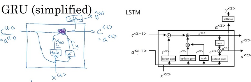
上图 四个小方块依次是 forget gate, update gate, tanh, and output gate
LSTM:
when use GRU or LSTM: isn’t widespread consensus in this(some problem GRU win and some problem LST win); Andrew:
- GRU is simpler model than LSTM and GRU is recently invention that maybe derived as simplification of more complicated LSTM model, easy to build much bigger network than LSFT,
- LSTM is more powerful and effective since it has three gates instead of two.
- LSTM is more historical proven choice, default first try. Now more and more team use GRU, more simpler but work as well.
Keras
Input shape = [batch size, # time steps, # dims for each time step]
e.g. batch_size = 30, # dims for each time step = 1, n_a (memory cell dimension) =3. So for each time step, the input size is 4 x 1 and memory cell dimension is 4 x 3
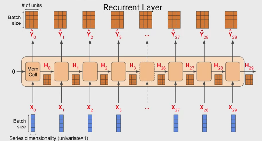
return_sequences=True: output all hidden state \(a^{<{t}>}\) as return output for LSTM layer
e.g. input with shape (num_seq, seq_len, num_feature). If we don’t set return_sequences=True, our output will have the shape (num_seq, num_feature), but if we do, we will obtain the output with shape (num_seq, seq_len, num_feature).
# return_sequences=False

inputs1 = Input(shape=(3, 1))
lstm1 = LSTM(1)(inputs1)
model = Model(inputs=inputs1, outputs=lstm1)
data = np.array([0.1, 0.2, 0.3]).reshape((1,3,1))
# make and show prediction

print(model.predict(data)) # [[0.05182764]]

#注: 因为weight initialization 不一样, 每次model.predict(data)值会不同


# return_sequences=True

lstm2 = LSTM(1, return_sequences=True)(inputs1)
model = Model(inputs=inputs1, outputs=lstm1)
print(model.predict(data)) #[[[0.00028653] [0.00073207  [0.00125595]]]
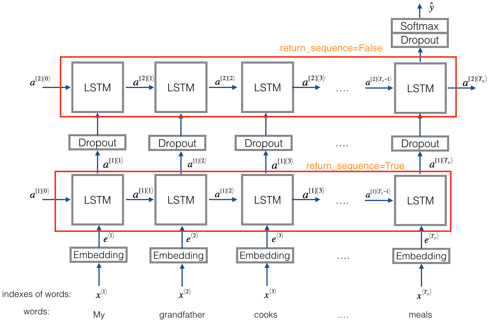
Besides, You must set return_sequences=True when stacking LSTM layers so that the second LSTM layer has a three-dimensional sequence input.
下面的code 中LSTM 会计算所有的 \(a^{\left[ 1\right] <{1}>}, a^{\left[ 1\right] <{2}>} ... a^{\left[ 1\right] <{T_x}>}\)
embeddings = Embedding(input_dim =vocab_size, output_dim = emb_dim)
X = LSTM(128, return_sequences=True)(embeddings)
- 下图底层的 LSTM 需要all pass hidden state output(activation) to 上层的LSTM as input. 所以
return_sequences=True - 上层LSTM 不generate output for each time step, so
return_sequences=False
return_state=True: LSTM layer that will provide the final hidden state activation \(a^{<T_x>}\) and the final state memory cell \(c^{<T_x>}\) .
- 如果设 return_sequences=False,
lstm=state_a, 都final hidden state activation - 如果设 return_sequences=True, 则
lstm为所有hidden state的activation,state_a为final state activation.lstm[-1]=state_a
inputs1 = Input(shape=(3, 1))
lstm, state_a, state_c = LSTM(1, return_state=True)(inputs1)
model = Model(inputs=inputs1, outputs=[lstm1, state_a, state_c])
data = np.array([0.1, 0.2, 0.3]).reshape((1,3,1))
print(model.predict(data))
# [array([[-0.11814568]], dtype=float32),

#   array([[-0.11814568]], dtype=float32),

#   array([[-0.20811582]], dtype=float32)]


lstm2, state_a, state_c = LSTM(1, return_sequences=True, return_state=True)(inputs1)
model = Model(inputs=inputs1, outputs=[lstm1, state_a, state_c])
data = np.array([0.1, 0.2, 0.3]).reshape((1,3,1))
print(model.predict(data))
# [array([[[-0.01104685], [-0.02694019], [-0.0446003 ]]], dtype=float32),

#  array([[-0.0446003]], dtype=float32),

#  array([[-0.10694385]], dtype=float32)]
TimeDistributed layer
Since we set return_sequences=True in the LSTM layers, the output is now a three-dimension vector (num_seq, seq_len, num_feature). If we input that into the Dense layer, it will raise an error because the Dense layer only accepts two-dimension input. In order to input a three-dimension vector, we need to use a wrapper layer called TimeDistributed. This layer will help us maintain output’s shape, so that we can achieve a sequence as output in the end.
比如下图红框的实现方式:
from tensorflow.keras.layers import  TimeDistributed,
X = TimeDistributed(Dense(1, activation = "sigmoid"))(X) # time distributed  (sigmoid)
LSTM Backprop
define \(d \Gamma_u, d \Gamma_f, d \Gamma_o, d \tilde c^{<{t}>}\) with respect to their argument inside sigmid or tanh function
\[\begin{align} \Gamma_u &= \sigma \left( \underbrace{ W_u \left[ a^{<{t-1}>}, x^{<{t}>} \right] + b_u}_{d \Gamma_u} \right) \\ \Gamma_f &= \sigma \left( \underbrace{W_f \left[ a^{<{t-1}>}, x^{<{t}>} \right] + b_f }_{d \Gamma_f} \right) \\ \Gamma_o &= \sigma \left( \underbrace{W_o \left[ a^{<{t-1}>}, x^{<{t}>} \right] + b_o }_{d \Gamma_o} \right) \\ \tilde c^{<{t}>} &= tanh \left( \underbrace{W_c \left[ a^{<{t-1}>}, x^{<{t}>} \right] + b_c }_{d \tilde c^{<{t}>}} \right) \\ c^{<{t}>} &= \Gamma_u \cdot \tilde c^{<{t}>} + \Gamma_f \cdot c^{<{t-1}>} \\ a^{<{t}>} &= \Gamma_o \cdot tanh\left(c^{<{t}>} \right) \\ y^{<{t}>} &= softmax\left( W_y c^{<{t}>} + b_y \right) \end{align}\]\(a^{<{t}>}\) is next layer input, so define \(da_{next} = \frac{dL}{da^{<{t}>}}\), as we know
\[\begin{align} \frac{\partial tanh\left(x \right)} {\partial x} &= 1 - tanh\left(x \right)^2 \\ \frac{\partial sigmoid\left(x \right)} {\partial x} &= \sigma\left( x\right) * \left(1-\sigma\left( x\right)\right) \end{align}\]when calculating partial derivative, need to include \(\frac{\partial L}{\partial c^{<{t}>}}\) and \(\frac{\partial L}{\partial a^{<{t}>}}\)
Define \(W_c \left[ a^{<{t-1}>}, x^{<{t}>} \right] + b_c\) as \(\phi\)
\[\begin{align} d\tilde c^{<{t}>} &= \frac{\partial L}{\partial c^{<{t}>}}\frac{\partial c^{<{t}>}}{\partial \tilde c^{<{t}>} } \frac{\partial \tilde c^{<{t}>} }{\partial \phi } + \frac{\partial L}{\partial a^{<{t}>}} \frac{\partial a^{<{t}>}}{\partial c^{<{t}>}}\frac{\partial c^{<{t}>}}{\partial \tilde c^{<{t}>} } \frac{\partial \tilde c^{<{t}>} }{\partial \phi } \\ &= \left( \frac{\partial L}{\partial c^{<{t}>}} + \frac{\partial L}{\partial a^{<{t}>}} \frac{\partial a^{<{t}>}}{\partial c^{<{t}>}} \right) \frac{\partial c^{<{t}>}}{\partial \tilde c^{<{t}>} } \frac{\partial \tilde c^{<{t}>} }{\partial \phi } \\ &= \color{fuchsia}{\left( dc^{<{t}>} + da^{<{t}>}*\Gamma_O^{<{t}>} * \left( 1- tanh\left( c^{<{t}>} \right)^2 \right) \right) * \Gamma_u^{<{t}>} * \left(1 - \left( \tilde c^{<{t}>} \right)^2 \right)} \\ \end{align}\]Define \(W_u \left[ a^{<{t-1}>}, x^{<{t}>} \right] + b_u\) as \(\phi\)
\[\begin{align} d\Gamma_u^{<{t}>} &= \frac{\partial L}{\partial c^{<{t}>}}\frac{\partial c^{<{t}>}}{\partial \Gamma_u^{<{t}>}} \frac{\partial \Gamma_u^{<{t}>}}{\partial \phi } + \frac{\partial L}{\partial a^{<{t}>}} \frac{\partial a^{<{t}>}}{\partial c^{<{t}>}}\frac{\partial c^{<{t}>}}{\partial \Gamma_u^{<{t}>} } \frac{\partial \Gamma_u^{<{t}>} }{\partial \phi } \\ &= \left( \frac{\partial L}{\partial c^{<{t}>}} + \frac{\partial L}{\partial a^{<{t}>}} \frac{\partial a^{<{t}>}}{\partial c^{<{t}>}} \right) \frac{\partial c^{<{t}>}}{\partial \Gamma_u^{<{t}>} } \frac{\partial \Gamma_u^{<{t}>} }{\partial \phi } \\ &= \color{fuchsia}{\left( dc^{<{t}>} + da^{<{t}>}*\Gamma_O^{<{t}>} * \left( 1- tanh\left( c^{<{t}>} \right)^2 \right) \right) * \tilde c^{<{t}>} * \Gamma_u^{<{t}>} * \left(1 - \Gamma_u^{<{t}>} \right)} \\ \end{align}\]Define \(W_f \left[ a^{<{t-1}>}, x^{<{t}>} \right] + b_f\) as \(\phi\)
\[\begin{align} d\Gamma_f^{<{t}>} &= \frac{\partial L}{\partial c^{<{t}>}}\frac{\partial c^{<{t}>}}{\partial \Gamma_f^{<{t}>}} \frac{\partial \Gamma_f^{<{t}>}}{\partial \phi } + \frac{\partial L}{\partial a^{<{t}>}} \frac{\partial a^{<{t}>}}{\partial c^{<{t}>}}\frac{\partial c^{<{t}>}}{\partial \Gamma_f^{<{t}>} } \frac{\partial \Gamma_f^{<{t}>} }{\partial \phi } \\ &= \left( \frac{\partial L}{\partial c^{<{t}>}} + \frac{\partial L}{\partial a^{<{t}>}} \frac{\partial a^{<{t}>}}{\partial c^{<{t}>}} \right) \frac{\partial c^{<{t}>}}{\partial \Gamma_f^{<{t}>} } \frac{\partial \Gamma_f^{<{t}>} }{\partial \phi } \\ &= \color{fuchsia}{\left( dc^{<{t}>} + da^{<{t}>}*\Gamma_O^{<{t}>} * \left( 1- tanh\left( c^{<{t}>} \right)^2 \right) \right) * c^{<{t-1}>} * \Gamma_f^{<{t}>} * \left(1 - \Gamma_f^{<{t}>} \right)} \\ \end{align}\]Define \(W_o \left[ a^{<{t-1}>}, x^{<{t}>} \right] + b_o\) as \(\phi\)
\[\begin{align} d\Gamma_o^{<{t}>} &= \frac{\partial L}{\partial c^{<{t}>}}\frac{\partial c^{<{t}>}}{\partial \Gamma_o^{<{t}>}} \frac{\partial \Gamma_o^{<{t}>}}{\partial \phi } + \frac{\partial L}{\partial a^{<{t}>}} \frac{\partial a^{<{t}>}}{\partial \Gamma_o^{<{t}>} } \frac{\partial \Gamma_o^{<{t}>} }{\partial \phi } \\ &= \left( \frac{\partial L}{\partial c^{<{t}>}}*0 + \frac{\partial L}{\partial a^{<{t}>}}\frac{\partial a^{<{t}>}}{\partial \Gamma_o^{<{t}>} } \right) \frac{\partial \Gamma_o^{<{t}>} }{\partial \phi } \\ &= \color{fuchsia}{da^{<{t}>}* tanh \left(c^{<{t}>}\right) * \Gamma_o^{<{t}>} * \left(1 - \Gamma_o^{<{t}>} \right)} \\ \end{align}\]So the derivatives for weights are:
\[\begin{align} \underbrace{dW_f^{\langle t \rangle}}_{a^{\langle t \rangle} \text{ x } \left( a^{\langle t-1 \rangle} + x^{\langle t \rangle} \right)} &= \underbrace{d\Gamma_f^{\langle t \rangle}}_{a^{\langle t \rangle} \text{ x } m} \underbrace{\begin{bmatrix} a^{\langle t-1 \rangle} \\ x^{\langle t \rangle} \end{bmatrix}^T}_{ m \text{ x } \left( a^{\langle t-1 \rangle} + x^{\langle t \rangle} \right)} \\ db_f^{\langle t \rangle} &= \sum_{batch} d\Gamma_f^{\langle t \rangle} \text{ where } db_f^{\langle t \rangle} \text{ dimension is } a^{\langle t \rangle} by 1 \\ dW_u^{\langle t \rangle} &= d\Gamma_u^{\langle t \rangle} \begin{bmatrix} a^{\langle t-1 \rangle} \\ x^{\langle t \rangle} \end{bmatrix}^T \\ db_u^{\langle t \rangle} &= \sum_{batch} d\Gamma_u^{\langle t \rangle} \text{ where } db_u^{\langle t \rangle} \text{ dimension is } a^{\langle t \rangle} by 1 \\ dW_c^{\langle t \rangle} &= d\widetilde c^{\langle t \rangle} \begin{bmatrix} a^{\langle t-1 \rangle} \\ x^{\langle t \rangle}\end{bmatrix}^T \\ db_c^{\langle t \rangle} &= \sum_{batch} d\widetilde c^{\langle t \rangle} \text{ where } d\widetilde c^{\langle t \rangle} \text{ dimension is } a^{\langle t \rangle} by 1 \\ dW_o^{\langle t \rangle} &= d\Gamma_o^{\langle t \rangle} \begin{bmatrix} a^{\langle t-1 \rangle} \\ x^{\langle t \rangle}\end{bmatrix}^T \\ db_f^{\langle o \rangle} &= \sum_{batch} d\Gamma_o^{\langle t \rangle} \text{ where } db_o^{\langle t \rangle} \text{ dimension is } a^{\langle t \rangle} by 1 \\ \end{align}\]Define
\[\begin{align} \color{red}{\phi_1} = W_u \left[ a^{<{t-1}>}, x^{<{t}>} \right] + b_u \\ \color{red}{\phi_2} = W_f \left[ a^{<{t-1}>}, x^{<{t}>} \right] + b_f \\ \color{red}{\phi_3} = W_o \left[ a^{<{t-1}>}, x^{<{t}>} \right] + b_o \\ \color{red}{\phi_4} = W_c \left[ a^{<{t-1}>}, x^{<{t}>} \right] + b_c \\ \end{align}\]Then
\[\begin{align} d a^{<{t-1}>} &= \frac{\partial L}{\partial \phi_1}\frac{\partial \phi_1}{\partial a^{<{t-1}>}} + \frac{\partial L}{\partial \phi_2}\frac{\partial \phi_2}{\partial a^{<{t-1}>}} + \frac{\partial L}{\partial \phi_3}\frac{\partial \phi_3}{\partial a^{<{t-1}>}} + \frac{\partial L}{\partial \phi_4}\frac{\partial \phi_4}{\partial a^{<{t-1}>}} \\ &= \color{fuchsia}{w_u^T d\Gamma_u^{<{t}>} + w_f^T d\Gamma_f^{<{t}>} + w_o^T d\Gamma_o^{<{t}>} + w_c^T d\widetilde c^{<{t}>}} \end{align}\] \[\begin{align} dx^{<{t}>} &= \frac{\partial L}{\partial \phi_1}\frac{\partial \phi_1}{\partial x^{<{t}>}} + \frac{\partial L}{\partial \phi_2}\frac{\partial \phi_2}{\partial x^{<{t}>}} + \frac{\partial L}{\partial \phi_3}\frac{\partial \phi_3}{\partial x^{<{t}>}} + \frac{\partial L}{\partial \phi_4}\frac{\partial \phi_4}{\partial x^{<{t}>}} \\ &= \color{fuchsia}{w_u^T d\Gamma_u^{<{t}>} + w_f^T d\Gamma_f^{<{t}>} + w_o^T d\Gamma_o^{<{t}>} + w_c^T d\widetilde c^{<{t}>}} \end{align}\] \[\begin{align} dc^{<{t-1}>} &= \frac{\partial L}{\partial c^{<{t}>} }\frac{\partial c^{<{t}>}}{\partial c^{<{t-1}>}} + \frac{\partial L}{\partial a^{<{t}>}}\frac{\partial a^{<{t}>}}{\partial c^{<{t}>}}\frac{\partial c^{<{t}>}}{\partial c^{<{t-1}>}} \ \\ &= \left( \frac{\partial L}{\partial c^{<{t}>} } + \frac{\partial L}{\partial a^{<{t}>}}\frac{\partial a^{<{t}>}}{\partial c^{<{t}>}} \right)\frac{\partial c^{<{t}>}}{\partial c^{<{t-1}>}} \ \\ &= \color{fuchsia}{\left(dc^{<{t}>} + da^{<{t}>} *\Gamma_O^{<{t}>}* \left(1 - tanh\left(c^{<{t}>} \right)^2 \right) \right) * \Gamma_f^{t}} \\ \end{align}\]Bidirection RNN
Unidirectional or Forward directional only RNN的问题,Motivated example:
- He said “Teddy bears are on sale”;
- He said “Teddy Roosevelt was a great President”.
Teddy都是第三个单词且前两个都一样,而只有第二句话的Teddy表示名字
Bidirection RNN(also defines a acyclic graph): forward prop从左向右 and 从右向左, 每个Bidirection RNN block还可以是GRU or LSTM的block. Lots of NLP problem, Birectional RNN with LSTM are commonly used(first thing to try)
- Bidirectional RNN is able to predict anywhere even in the middle of a sequence by taking into account information potentially from the entire sequence
- for NLP, when you can get entire sentence all the same time, standard BRNN algorithm is very effective
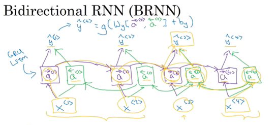
Disadvantage: 需要entire sequence of data before you can make prediction; 比如speech recognition: 需要person to stop talking to get entire utterance before process and make prediction
Deep RNNs
- \(a^{\left[ l \right] <{t}>}\) denote the activation with layer l over time t
- \(w_a^{\left[ 1 \right]},b_a^{\left[ 1 \right]}\) used for every computation in first layer; \(w_a^{\left[ 2 \right]},b_a^{\left[ 2 \right]}\) used for every computation in layer 2;
- 每个block 也可以是GRU, 也可以是LSTM, 也可以build deep version of bidirectional RNN,
- 在output layer也可以有recurrent layers stack on top of each other, 下图中\(y^{<{1}>}\)的上边,have a bunch of deep layers that are not connected horizontally, then finally predict \(y^{<{1}>}\),
- Disadvantage: computational expensive to train
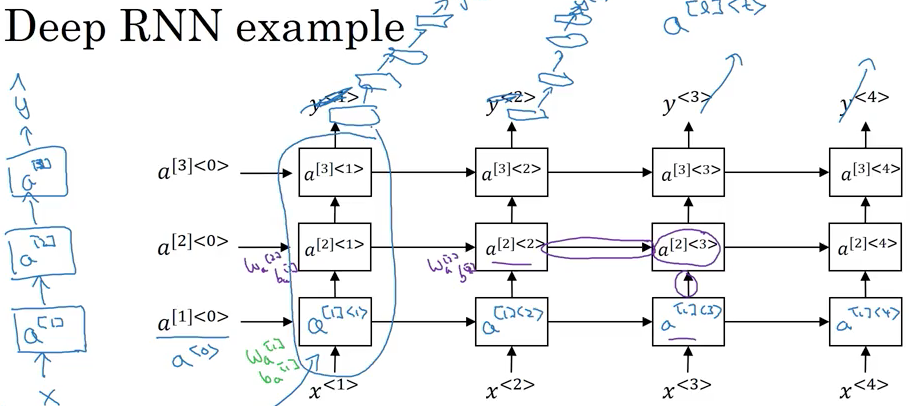
比如计算\(a^{\left[{2}\right]<{3}>}\): \(a^{\left[{2}\right]<{3}>} = g\left( W_a^{\left[ 2 \right]} \left[a^{\left[{2}\right] <{2}>}, a^{\left[ {1} \right] <{3}>} \right] \right)\)
For RRN, 三层已经是very deep, don’t see many deep recurrent layers that are connected in time, whereas there could be many layers in a deep conventional neural network.
2. NLP & Word Embedding
Word Embedding
Word Embedding: The way of representing words.
One hot vector Disadvantages:
- it deoesn‘t alow an algorithm to easily generalize across words
- 10000中(10000是字典),只有1个为1表示这个词,不能表示gender. age, fruit…,
- any dot product between any two different one-hot vector is zero and Eludian distance between any pair is the same. e.g. King vs Apple and Orange vs Apple dot product are the same(zero)
- e.g. orange juice then should know Apple ___, juice is popular choice since orange and apple is similar
- Computational expensive, high dimensional vector
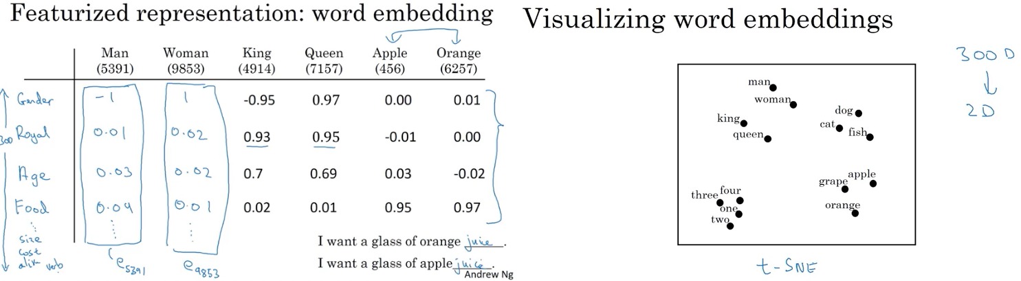
- featurized representation (embeddings) with each of these words, 比如一个 vocabulary dictionary size 10000, 而每个word 比如有300 feature, feature vector size = 300,
- use \(e_{5391}\) denote the embedding for Man, 5391 is the position of one hot vector equal to 1
- Featurized representaion will be similar for analogy. e.g. Apple vs Orange, Kings vs Queens
- In practice, feature(word embedding) that used for learning won’t have a easy interpretation like gender, age, food …
- It allow to generalize better across different words
- E,g, “apple farmer” vs “durian cultivator”: If have a small trianing set for named entity recognition, “durian” or “cultivator” might bno in training set. But if learn from embedding, it can still generialize to tell durian is a fruit and cultivator is a farmer
- T-SNE(complicated, non-linear mapping): take 3000vector visualize to 2-Dimensional space, analogy tends to close (上图右侧)
- Word Embedding can be learned from very large unlabeled training datasets (~1 billion - 100 billion), then can find apple and durian, farmer and cultivator are kind of similar
- Or can download pre-trainined embedding online
- Take the learned word embedding from step 1 to new task with much smaller labeled training set. (maybe ~ 100k)
- carry out transfer learning to a new task such as named entity recognition
- can use relative lower dimensional feature vector from word embedding (maybe ~300 dense vector rather than 10000 of one hot vector)
- Optional: continue to fine-tune(adjust) word embeddings with new data(only your task dataset is really large)
Advantage: word embeddings can allow to be carried out with a relatively smaller labeled training set
- used for many NLP Application: such as named Entity Recognition, text summarization, co-reference resolution, parsing.(transfer from task A to some task B, when A has large dataset and B has relative smaller dataset) Less useful for language modeling, machine traslation especially having large dataset
Difference between face recognition and word embedding:
- face recognition can have neural network to compute an encoding(embedding) for any picture even the picture haven’t seen before
- word embedding, 比如 we have a fixed 10000 word vocabularies, only learn those 10000 word embedding in our vocabularies (fetaures)
Word Embedding Applications: can be learn from large text corpus
- learn analogy such as boy - girl as man - woman
- learn capital. such as Ottawa: Canada as Nairobi : Kenya
- learn Yen: Japn as Ruble: Russia
- learn Big: Bigger as Tall: Taller
Cosine Similarity
比如 \(e_{man} - e_{woman} \approx e_{king} - e_{?} \text{用similarity function}\)
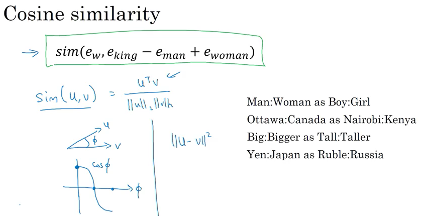
Find a word w to maximize the similarity between \(e_{w}\), and\(e_{king} - e_{man} + e_{woman}\). In practice, it works by finding a word to maximize the similarity and can get the exact right answer. And count the analogy is correct only get exact word right
\[argmax_{w} sim\left( e_{w}, e_{king} - e_{man} + e_{woman} \right)\]- \(u^Tv\) inner product, if u and v are very similar, it tends to be large. 因为\(u^Tv\)表示他们的夹角(cos)
- or use Euclidian distance: \({\|u-v\|}^2\) 通常 measure dissimilarity than similarity. if measure similiarity, should take \(-{\|u-v\|}^2\) Cosine Similarity being used often.
- Difference between cosine and Euclidian distance similarity is how to normalize the length of the vectors u and v
Embedding Matrix:
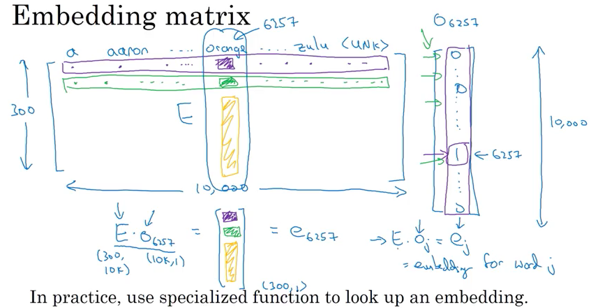
Goal: learn 300 features by 10000 words vocabulares embedding matrix( 300 x 10000).
- Intialize E randomly and use gradient descent to learn all the parameter in E.
- \(E * o_j = e_j\) , \(o_j\) is one-hot vector and \(e_j\) is embedding vector
- In practice, not use matrix multiplication (\(E * o_j = e_j\) ) to get embedding vector,not efficient, 用just lookup word emdding matrix column e
- e.g.
Learn Word Embeddings
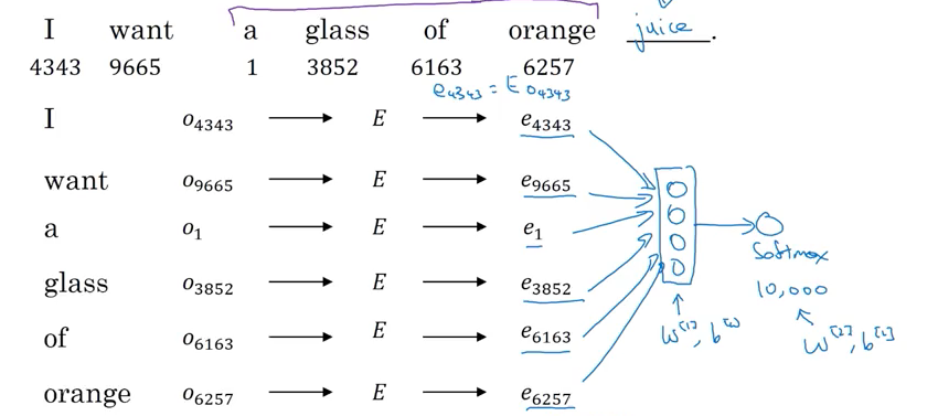
Fixed window: 比如I want a glass of orange ___ , e.g. fixed window size = 4
- 预测是juice,代入前四个words, a glass of orange 的 one-hot vector
- lookup get 300 dimension embedded vector (e.g \(e_{4343}, e_{9665}\)) from embedding-matrix (\(E\): is the same for all training examples)
- Then feed those Embedding vectors to a neural network and then feed to a softmax which output 10k output.
- can use backprop to perform gradient descent to maximize likelihood of training set
- repeatedly predict nxt word given four words in a sequence in text corpus
Advantage: can deal with arbitrary long 句子,因为input size is fixed
- it can learn similar embedding for orange and apple
Ohter Context / target pairs:
- Input: 4 Words on left & right. predict: word in middle
- Input: Last One word. predict: next word
- Nearby one word: Input: saw the word “glass”, Predict: then there’s another words somewhere close to “glass“(an example Skip Grams, it works remarkably well)
Word2Vec Skip-grams
比如句子: I want a glass of orange juice to go along with my cereal;
- 先 pick context word e.g. orange,
- Then randomly pick another word within some window as target word 比如context word前后的5个或者10个词;
- e.g 1. context: orange -> target: juice;
- e.g 2. context: orange -> target: glass;
- e.g 3. context: orange -> target: my;
- Not a easy learning problem, because too many different words can be chosen within windows
- Goal: Not to do well on the supervised learning (predict target from context). Instead using learning problem to learn a good embedding.
- Supervised learning: Learning the mapping from content C (e.g. orange (word index 6257) ) to target t (e.g. juice (word index 4834) )
Model:
\[\require{AMScd} \begin{CD} \underbrace{O_c}_{\text{ one hot vector}} @>>> \underbrace{E}_{\text{embedding matrix}} @>>> \underbrace{e_c}_{\text{embeding vector}} @>>> softmax @>>> \hat y \end{CD}\]where softmax is as below, \(\theta_t\) is parameter associated with output t, used to predict the chance of word t being label
\[p(t |c) = \frac{ \theta_t^T e_c }{ \sum_{j=1}^{10,000} { e^{ \theta_j^T e_c } } }\]Loss function: where \(y_i\) is one hot vector; \(y_i\) and \(log\hat{y_i}\) both are 10000 dimenional \(y_i log\hat{y_i}\), is dot product
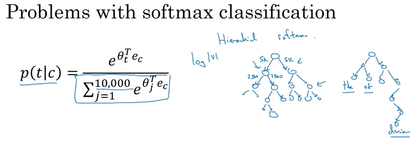
\[L \left(\hat y , y \right) = - \sum_{i=1}^{10,000} { y_i log\hat{y_i} }\]Problem with softmax classification:
- computationtal expensive, every time need to calculate the sum of all vocabulary \(\sum_{j=1}^{10,000} { e^{ \theta_j^T e_c } }\) if use vocabulary size is 1 million, it gets really slow
Solution Hierarchical Softmax, link:
- 如下面图,instead of carrying 10000 all the time , tell if target word in
[0, 5000)or[5000, 10000]in vocabulary, then find if in[0,2500), or[2500, 5000), then find the target node and calculate the probability without sum over all vocab size to make a single prediction - 每一个parent 记录所有的softmax的和of all childs; complexity: \(log \mid v\mid\) ;
- In practice, don’t use perfectly balanced tree or symmetric tree, more common word on the top, less common word on deeper of the tree(because don’t need to go to that deep frequently), 如下图右侧的图
How to choose/sample context word c:
- if uniformly random sample from training corpus, 可能会选择很多the, a, of, and, to,但我们更想让model训练比如orange, durian这样的词. want to spend some time updating even less common words embedding like durian
- In practice, the distribution of words is not entirely uniform. Instead, there are different heuristics that you could use to balance out common words together with less common words
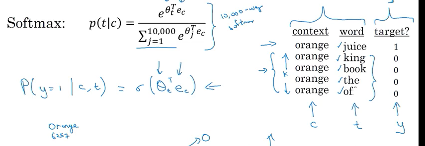
Negative Sampling
Create a new supervise learning problem: Given pair word: orange & juice. Is this a context - target pair?
- Generate positive example: Sample(choose) a context word, look around a window of e.g. \(\pm 10\) words and pick a target word
- 比如: “I want a glass of orange juice to go along with my cereal”. pick “orange” as context word, then choose “juice” as target word
- Generate negative example: take the same context word, then pick k word randomly from the dictionary/vocabulary.
- e.g. pick context word as “orange”, then choose word “king” from vocabulary
- It is okay if the word chosen from vocabulary also appear in the window. e.g. 下面的 “of”
- create supervise learning problem, x is context and word, y as label. Try to distinguish the distribution from chosen near context and chosen from dictionary
k = [5,20]for small dataset,k = [2,5]for large dataset
| Context | Target | target? |
|---|---|---|
| orange | juice | 1 |
| orange | king | 0 |
| orange | book | 0 |
| orange | of | 0 |
Model: to define a logistic regression, the chance \(y=1\) given the context and target pair.
\[P\left( y = 1 \mid c,t \right) = \sigma \left( \theta^T e_t \right)\]where \(\theta_t^{T}\) parameter vector theta for each possible target word, \(e_c\) for embedding vector.
- For every positive example, having k negative example to train the logistic regression model
- Turn into 10000 binary classification problem(每一个problem 对应一个 \(\theta_t\) ) instead of 10000 way softmax which is expensive to compute (given orange, predict 10000 all vocabulary).On every iteration, only train k+1 example(1 positive example, k randomly negative example)
- Select samples: If you choose words 根据its empirical frequence 可能有很多词 如 the, of, and; or sample uniformly random based on vocab size \(\frac{1}{\mid V \mid}\). It is also non-representative of the distribution of English word use \(P(W_i) = \frac{ f \left(w_i \right)^{3/4} }{ \sum_{j=1}^{10,000} { f\left(w_i \right)^{3/4} } }\) 这个分布选取, \(f \left(w_i \right)\) is frequency of each word in English text
- Or can use pre-trained embedding vectors as starting point
GloVe
Glove: global vector for word presentation
- \(X_{ij}\) = the number of times j (target) appears in context of i
- j 在i的上下文出现多少次; 如果上下文是前后10个词的话, 也许得到symmetric relationship \(X_{ij} = X_{ji}\); 当如果只选word before it, may not get symmetric relationship
- \(X_{ij}\) is the count how often do words i and j appear close to each together
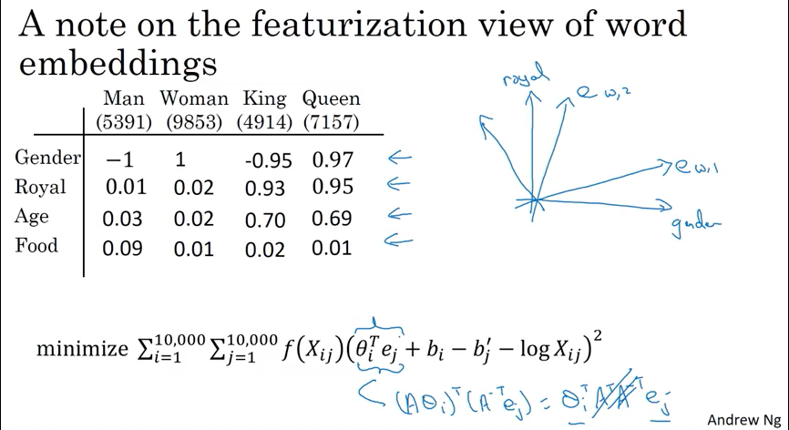
Objective function:
\[minimize : \sum_{i = 1}^{10,000} \sum_{j = 1}^{10,000} {f\left(X_{ij} \right) \left( \theta_i^T e_j + b_i + b_j' - log X_{ij} \right)^2}\]- want to tell how related word i and j (target and content) / how often they occur with each other
- \(f\left(X_{ij} \right)\) is weighting term,
- 当 \(X_{ij} = 0\),\(f\left(X_{ij} \right) = 0\) , 避免 当 \(X_{ij} = 0\)时, \(log\left( 0\right)\) undefined,
- also, \(f\left(X_{ij} \right)\) give more weight to less frequent word like durian, and give less weight for common word like this, is, of, a
- \(\theta_i\), and \(e_j\) are symmetric(could reverse then can get the same optimization objective)
- Initialize \(\theta\), and \(e\) both uniformly random and perform gradient descent to minimize the objective. Take average when finish training \(e_w^{final} = \frac{\left( e_w + \theta_w \right)} {2}\)
- \(\theta\), and \(e\) play the symmetic roles unlike others previously play different role
- Even though the objective function is simple, it works

Cannot 保证individual components of embedding 是可以解释的(interruptable). The first feature (\(e_{w,1}\)) might be combination of age, gender, and royal. parallelogram(平行四边形) for analogies still works despite potentially arbitrary linear transformation of the features.
\[\left( \theta_i^T e_j \right) = \left( A \theta_i\right)^T \left(A^{-T} e_j \right) = \theta_i^T \cancel{A A^{-T}} e_j\]which prove that axis used to represent the features will be well-aligned with what might be easily humanly interpretable axis
Embedding Application
Sentiment Classification
Chanllenge: not have a huge dataset, 1 millon is not common, sometimes around 10000 words
If embeding matrix is trained from large training set(e,g 1 million), it can learn feature for infrequent word even the word not in Sentiment classification training set (比如 durian not in Sentiment classification training dataset, but e learned from word embedding, then can better generalize result)
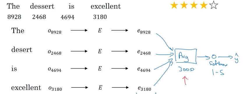
Method 1: Simple Sentiment Classification Model
- use one hot vector, lookup embedding matrix then get embedding vector
- If embedding matrix is trained on large dataset, it allows to take a lot of knowledge even from infrequent word, and apply them to your problem even words not in your labeled training set
- then get all embedded word in a word, then take average or sum of all embedded vector as input layer (
300 x 1feature vectors )- because take average, it works for review sentences that short or long
- Pass embedding vectors from step 2 to a softmax and output \(\hat y\) (5 outcomes, 1-5 stars)
Problem: Ignore order :比如: “completely lacking good taste, good service an good ambience”: 即使有3个good,也是negative review.
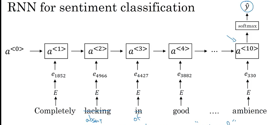
Method 2: RNN for sentiment Classification many-to-one architecture :
- use one hot vector, lookup embedding matrix then get embedded vector e.g \(e_{8928}\)
- then feed embedding vectors into RNN. The job of RNN is to compute the representation at last time step for \(\hat y\)
- it can train to realize “lack of good” and “not good” is negative review
- Because word embedding can be trainied from a much larger data set, this will do a better job to generalizing even new words that not seen in labeled training set, e.g. “absent of good”, and absent not in labeld training set -> negative review
Debiasing Word Embeddings
- bias here not meaning bias/variance, means the gender, ethnicity, sexual orientation bias.
- 比如 man: programmer as Woman: Homemaker; 比如 man: Doctor as Mother: Nurse;
- Word embeddings可以reflect gender, ethnicity ages… bias of text used to train model as bias is related to socioeconomic status
- we try to change learning algorithm to eliminiate these types of undesirable biases
- The bias the model pick up tend to reflect the biases in text written by people
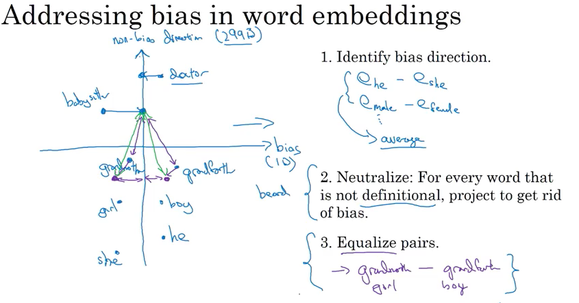
Address bias:
- Identiy bias direction-
- 比如用 embeded vector \(e_{he} - e_{she}; e_{male} - e_{female}\)… then averge them(In original paper, use Singular Value Decomposition instead of average)
- average 得到bias direction(1 dimension. In original paper, bias direction can be higher than 1 dimensional), 垂直的bias direction是 non-bias direction(if bias is 1 dimension, non-bias is 299 dimension)
- Neutralization:
- definitional e.g gender is intrinsic in definition 的是grandmother, grandfather, non-definitional比如 doctor, babysitter
- For non-definitional words, project them onto non-bias direction to get rid of bias;
- 对于如何选取什么word neutralized,, e,g, doctor is not gender specific need to be neutralized, whereas grandfather / grandmother should not neutralized (made gender specific). 再比如 Beard should be close to male not female
- author;train a classifier to try to figure out 什么word是definitional(e.g. 什么word是gender specific) 什么不是; 大多数英语单词都是not definitional的
- Equalize pairs:
- 比如 grandfather vs grandmother, boy vs girl-> want to only difference in embedding is gender, 比如下图中 distance between babysitter’s projection and grandmother is smaller than the distance between babysitter’s projection and grandfather, which is a bias;
- 所以移动grandfather 和 grandmother to pair points (到距离Non-bias axis的距离一样的点);
- 选取equalized pairs不会很多,可以hand-picked
3. Sequence Models & Attention Mechanism
Encoder-Decoder
Machine translation:
- RNN encoder network can be built as GRU or LSTM; French word(需要被翻译的) one word each time as input, then RNN generates a vector that represents the input sentence.
- Decoder netork take the encoding output by encoder network as input. Then generate translation one word at time( 一个一个output 翻译的单词). Then at the end of sentence, decoder stops.
- This model works decently well, given enough pair French and English sentences
- Difference from synthesizing novel text using language model: 不需要randomly choose translation, want the most likely translation.
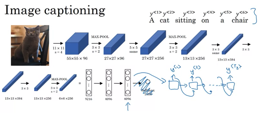
Applications: Image captioning
- AlexNet gives 4096 dimensional feature vector(softmax 之前) to represent the picture. The pretrained AlexNet can be Encoder network for image
- Feed 4096 dimensional feature vector into RNN to generate the caption one word at a time.
- This model works well for image captioning, especially the caption is not too long
Pick the Most likely Sentence
Machine translation as building a conditional language model. Instead of modelling probability of any sentences, it model the probability of output English translation condition on some input French sentence.
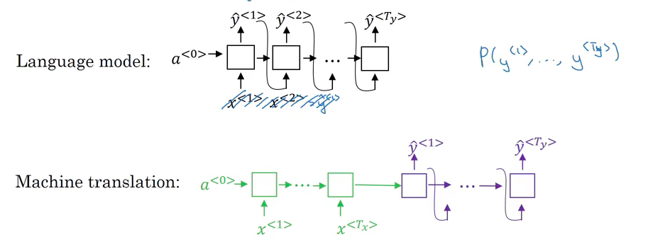
\[P \left( y ^{<{1}>}, y ^{<{2}>},\cdots, y^{<{T_x}>}\vert x ^{<{1}>}, \cdots, y ^{<{T_x}>} \right)\]- Language model use previous generated \(\hat y^{<{t-1}>}\) as next time input \(x^{<{t}>}\).Decoder network looks very similar to Lanuage model except \(a^{<{0}>}\) of decoder network are from encoder network instead of a vector of all zeros
- can think machine translation as building a conditional language model.
Finding the most likely translation : 不能用random sample output from \(y^{<{t-1}>}\) to \(y^{<{t}>}\), 有时候可能得到好的,有时候得到不好的翻译; Instead should find y that maximized the conditional probability. The most common algorithm is Beam Search
\[\underbrace{arg max}_{y^{<{1}>}, \cdots, y^{<{T_y}>}} P\left( y^{<{1}>}, \cdots, y^{<{T_y}>} \vert x \right)\]e.g. “Jane visite l’Afrique en septembre”, by random sample, may get below translation
- Jane is visting Africa in September
- Jane is going to be visiting Africa in September (Akward)
- In September, Jane will visit Africa
- Her African friend welcomed Jane in September (bad translation)
The goal should maximize the probability \(P \left( y ^{<{1}>}, y ^{<{2}>},\cdots, y^{<{T_x}>}\vert x \right)\)
Why not Greedy Search
- after pick first word that most likely,then choose 概率最高的第二个单词,再选择概率最高的第三个单词
- because need to maximimize joint probability \(P \left( y ^{<{1}>}, y ^{<{2}>},\cdots, y ^{<{T_x}>} \vert x \right)\), 这么选出的word组成的句子 不一定是接近最大的joint probability 的句子;
- 比如Jane is visiting Africa in September: perfect翻译, 但是greedy翻译出来 Jane is going to be visiting Africa in September. 因为
P(Jane is going) > P( Jane is visiting)(因为going is more frequent)
- 比如Jane is visiting Africa in September: perfect翻译, 但是greedy翻译出来 Jane is going to be visiting Africa in September. 因为
- The total number of combinations is expotentially large. E.g. vocabulary size is 10000, and 10 words in a sentence, then there are \(10000^{10}\) possibility. That’s way to use an approximate search algorithm. The algorithm are not always succeed. It will try to pick sentence y to maximize the \(\underbrace{arg max}_{y^{<{1}>}, \cdots, y^{<{T_y}>}} P\left( y^{<{1}>}, \cdots, y^{<{T_y}>} \vert x \right)\). It usually do a good job.
Beam Search
Beam Search Algorithm (a approximate/heuristic search algorithm), B = beam width: 不像greedy search 每次只考虑最大可能的一个词,beam search 会考虑最大可能的B个词; 注: 当B=1, 相当于greedy search.
- Every step, instantiate B copies of network to evaluate partial sentence fragments and output
- Beam Search usually find much better output sentence than greedy search
- 不像BFS, DFS. Beam Search runs faster, but is not guaranteed to find exact maximum for \(arg \underbrace{max}_{y} P\left(y \vert x \right)\)
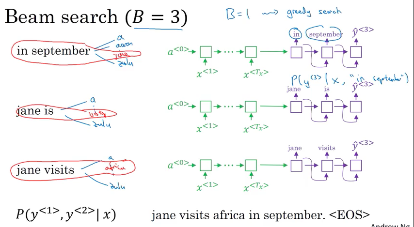
Example: B = 3 (case insensitive in this example)
- Step1: The first step of decoder network a softmax \(P\left(y^{<{1}>} \vert x\right)\), find in, jane, september most likely 3 possibility based on \(P\left(y^{<{1}>} \vert x\right)\), keep
[in, jane, september]in memory - Step2: using decoder network to evulate \(P\left(y^{<{2}>} \vert y^{<{1}>}, x\right)\) separately given the \(\hat y_{1} = in\), \(\hat y_{1} = jane\), and \(\hat y_{1} = september\), to maximize \(P\left(y^{<{1}>}, y^{<{2}>} \vert x\right) = P\left(y^{<{1}>} \vert x\right) P\left(y^{<{2}>} \vert y^{<{1}>}, x\right)\)
- 比如字典有10000个词,考虑来自step1三个词作为开始,every step consider maximized only 10000*3个词, then pick top3; 比如发现最大可能性的三个词 [In september, jane is, jane visit] -> reject september 作为第一个词的可能
- Step 3: decoder ends at when output end-of-sentence (
EOS) token e.g. Jane visits africa in september
Length normalization,
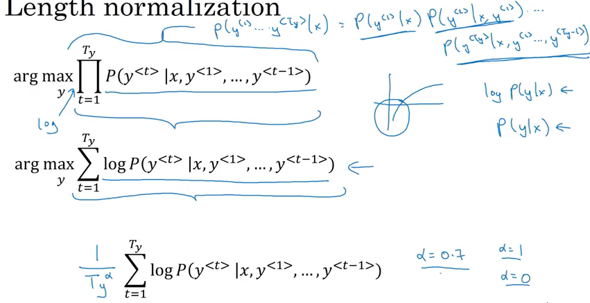
Problem 1: 可能概率的乘积越来的越小, mutliply the number less than 1 (probability less than 1) result in tiny number which can result in numerical underflow, floating part representation maynot store accurately
\[\begin{align} arg \underbrace{max}_{y} \prod_{t=1}^{T_y} P\left( y^{<{t}>} \vert x, y^{<{1}>} , \cdots, y^{<{t}>} \right) &= P\left( y^{<{1}>}, \cdots, y^{<{T_y}>} \vert x, \right) \\ &= P\left( y^{<1>} \vert x \right) P\left( y^{<2>} \mid x, y^{<1>} \right) ... P\left(y^{<{t}>} \vert x, y^{<{1}>}, y^{<{2}>}, \cdots, y^{<{t-1}>} \right) \end{align}\]Solution: In practice, instead of maximizing product, we maximize sum of log probability to get more stable numerical value less prone to rounding error. Log functon is strictly monotonically increasing function, maximizing log probability is the same as maxmizing probability
\[arg max_{y} \sum_{y=1}^{T_y} log P\left(y^{<{t}>} \vert x, y^{<{1}>}, y^{<{2}>}, \cdots, y^{<{t-1}>} \right)\]Problem 2: 可能prefer更短的句子, 因为probability都是小于1,句子越长概率乘积越小,同样log都是小于0,句子越长sum越小
Solution: use normalized log likelihood objective function,除以句子长度, reduce penalty of otput longer translation.
- maybe \(\alpha = 0.7\), 表示 \(T_y\) 的0.7 次方. 0.7是between full normalization and no normalization;
- 当\(\alpha = 1\), complete normalize by length;
- 当\(\alpha = 0\), \(\frac{1}{T_y^{\alpha}} = 1\): not normalized at all.
- 同时alpha也可以作为hyperparameter 用来tune
- 句子越长, \(\frac{1}{T_y^{\alpha}}\)越小 且 \(\sum_{y=1}^{T_y} log P\left(y^{<{t}>} \vert x, y^{<{1}>}, y^{<{2}>}, \cdots, y^{<{t-1}>} \right)\) is negative, 所以下面formula 得到的值越大
Run Beam Search
- Run Beach Search for sentence lengths up to \(T_y\) 1,2,…,30 steps
- keep track of top 3 possibilies for each of these possible length (比如lengths from 1:30 and beam = 3, 共90个选择),
- pick the one 有最高score的( highest normalized log likelihood objective) 作为final translation output
How to choose Beam width B? production system around 10; 100 consider be large; 1000, 3000是not common的, 用越来越大的B, often diminishing returns; 比如gain很大 当beam从1->3->10, 但是gain不是很大了, 当beam 从1000->3000,
- large B: pro: better result, con: slower, memory requirement grows
- small B: pro: run faster and memory requirement lower, con: worse result
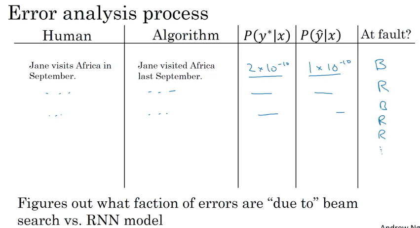
Beam Search Error Analysis
Example:
Jane visite l’Afrique en septembre.
Human 翻译: Jane visits Africa in September (\(y^{*}\)) better
Algorithm 翻译: Jane visited Africa last September (\(\hat y\))
Is it RNN error or beam search error? Can get more data or incream beam width increase performance? Increasing beam width won’t hurt bug might not get the same result as you want
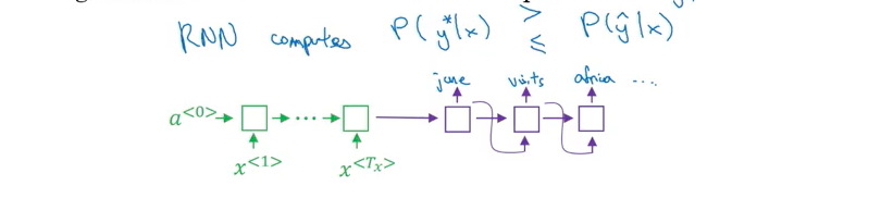
用RNN 计算 \(P\left( y^{*} \vert x \right)\) (plugin human translation result into decoder to calculate ), \(P\left( \hat y \vert x \right)\), 可以用length normilization when calculating probability (短的sentence high probability)
- Case 1: \(P \left( y^{*} \vert x \right)\) > \(P\left(\hat y \vert x \right)\) : Beam choose \(\hat y\), 但是 \(y^{*}\) attains 更高的 P(y|x); Beam search is at fault (beam search job: choose maximized probability )
- increase beam width
- Case 2: \(P\left( y^{*}\vert x \right)\) <= \(P\left(\hat y \vert x \right)\): \(y^{*}\) better translation than \(\hat y\), 但是 RNN预测相反, RNN (objection function) is at fault
- add regulartion, get more training data, try different network architecture etc
Bleu Score
- given French sentence, 有几个英语翻译,how to measure multiple equally good translation? Bleu: Bilingual evalutation understudy.
- Bleu Score: Given machine generated translation, compute a score that measures how good is the machine tranlation
- if machine tranlation close to references provided by human -> High Score
- human provided reference is part of dev/test set, to see if machine generated word appear at least once in human provided reference
- is pretty good single real number evaluation metric
- In practice, few people implement from sratch, many open source implementations
- Bleu Score 应用于machine translation or 给图片起标题 (image caption), there exists some outputs equally good(比如下面example 的reference 1,1); not use in speech recognition, 因为speech recognition一般都有one ground truth
e.g. An extreme example:
- French: Le chat est sur le tapis
- Reference 1: The cat is on the mat.
- Reference 2: There is a cat on the mat.
- Machine Translation(MT) output: the the the the the the the.
Unigram
-
Precision: \(\frac{\text{(count of every words either appear in reference 1 or reference 2}}{\text{total words}}.\)
- 上面例子 MT = \(\frac{7}{7} = 1\) ( not a particularly useful measure, it seems that MT output has a high precision)
-
Modified Precision: \(\frac{\text{(credit only up to maximum appearance in one reference sentence)}}{\text{total words}}.\)
- 上面MT翻译中 the 在1中出现了2回, MT = \(\frac{2}{7}\), 分子是 (numerator): the maximum number of times “the” appears in reference 1 or 2 (“the” appear twice in reference 1, “the” appear once in reference 2)
- numerator: max count/clip count, 分母(denominator)是 the total count of number words in machine tranlated sentence
Bigram
e.g. An extreme example:
- French: Le chat est sur le tapis
- Reference 1: The cat is on the mat.
- Reference 2: There is a cat on the mat.
- MT output: the cat the cat on the mat.
Bleu score on bigrams: bigram 两个两个词连在一起看有没有在reference 1 or 2中出现
Count column 指的是在 the number of appearance in machine translation. Count Clip is the maximum number of appearance of the pair either in reference 1 or reference 2
| Context | Count | Count Clip |
|---|---|---|
| The cat | 2 | 1 |
| cat the | 1 | 0 |
| cat on | 1 | 1 |
| on the | 1 | 1 |
| the mat | 1 | 1 |
Modified Precision on unigram, bigram, n-gram measure the degree how similar / overlap the machine translated sentences with human references. 如果机器翻译的跟reference 1 or reference 2完全一样, \(P_1\) and \(P_n\) 都等于1
| unigram | n-gram |
|---|---|
| \(\displaystyle p_1 = \frac{ \sum_{unigram \in \hat y }^{} { Count_{clip} \left( unigram \right)} }{ \sum_{unigram \in \hat y }^{} { Count\left( unigram \right)} }\) | \(\displaystyle p_n = \frac{ \sum_{\text{n-gram}\in \hat y }^{} { Count_{clip} \left( \text{n-gram} \right)} }{ \sum_{\text{n-gram}\in \hat y }^{} { Count\left( \text{n-gram} \right)} }\) |
Combined Blue score: \(p_n\) Bleu score on n-grams only, such as \(p_1, p_2, p_3, p_4\)
\[BP exp\left( \frac{1}{4} \sum_{n=1}^4 {P_n} \right)\]- BP(brevity penalty) if output is short, 容易得到high precision Bleu Score; BP is adjustment factor 避免too short. The brevity penalty penalizes generated translations that are too short compared to the closest reference length with an exponential decay. The brevity penalty compensates for the fact that the BLEU score has no recall term.(recall: 是不是reference 中的正确都predict了,referenece length > candidate length, no penalty )
Attention Model
problem with encoder & decoder network:
- given long sentence, encode 只能读完句子所有内容后, 再通过decoder进行翻译输出;(different from human translation which translate sentence part by part and difficult to memorize the whole long sentence)
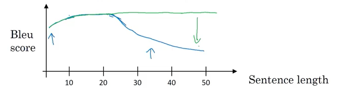
- Encoder-Decoder network(下图的蓝线) 对于 短的句子和很长的句子效果不好。Short sentence hard to translate right and long sentence is diffcult for neural network to memorize a super long sentence.
- Attention Model: translate like human, looking at part of sentence at a time and with Attention model, machine translation systems performance can look at 下图的绿线
- Attention model not only used in machine translation, also used in many other applications as well
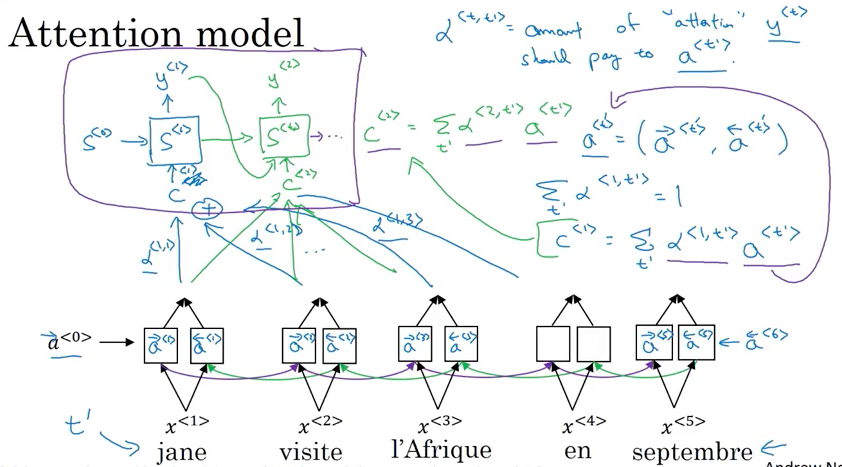
E.g French translate to English
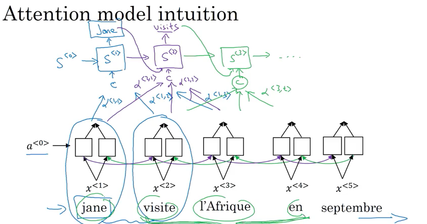
- 用bidirectional RNN but not doing the word by word translation. By using BRNN, for each words, can compute rich set of features about the words and surrounding words in every position
- Use another RNN generate English translation. Instead of using \(a^{<{t}>}\) to denote activation, use \(s^{<{t}>}\) to denote activation. \(s^{<{2}>}\) 需要 \(s^{<{1}>}\) (generate的第一个词) 作为input。
- When generate first output/word, only look at words close by. What attention computing is a set of attention weight, denote by \(\alpha\)
- \(\alpha^{<{1,2}>}\) denote how much attention pay to second piece information from BRNN as input to generate first word using RNN
- \(\alpha^{<{2,1}>}\) denote how much attention pay to first piece information from BRNN as input to generate second word using RNN
- \(\alpha^{<{t,t'}>}\) tell when generate t-th English word how much attention should pay to t’-th French word. This allow every time step to look only with a local window of French sentence to pay attention to when generating specific English word
- To generate second words, also put the first generated word “Jane” as input besides \(\alpha^{<{2,1}>}, \alpha^{<{2,2}>}, \alpha^{<{2,3}>}\)
- 最后generate
EOS - \(\alpha^{<{3,t}>}\) is depended on previous step activation \(s^{<{2}>}\) and BRNN activation \(\overrightarrow a^{<{t}>}\), \(\overleftarrow a^{<{t}>}\)
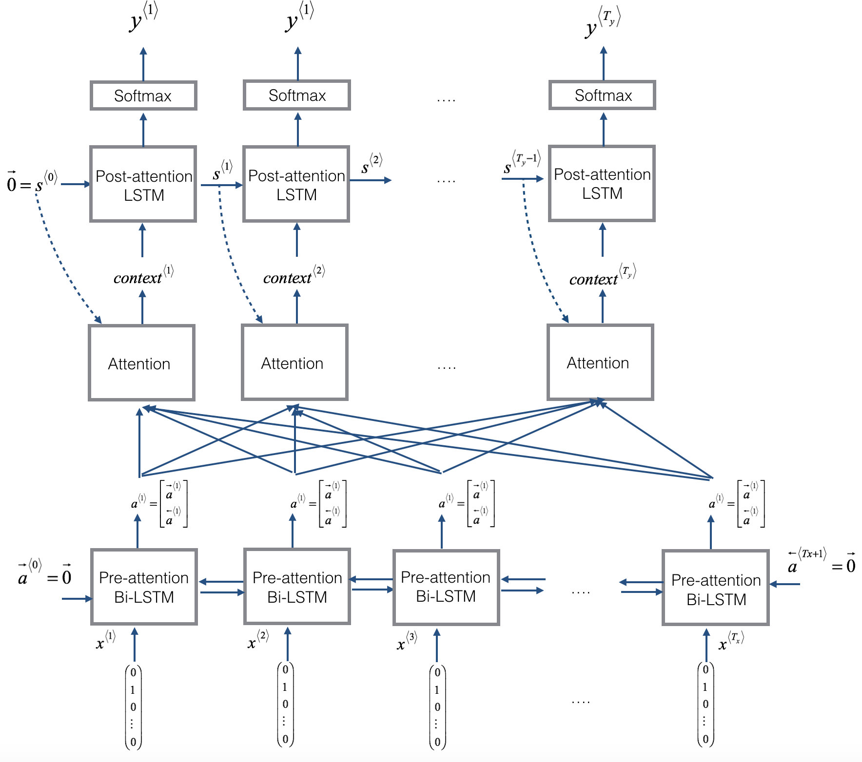
Attention Model Training
- 下面network 是BRNN(or Bidirectional GRU or Bidirectional LSTM) to compute features for each word, 上面network 是standarad RNN
- 下图中\(\overrightarrow a^{<{0}>}\), \(\overleftarrow a^{<{6}>}\)是zero vector(不是input sequence中的), 用\(a^{<{t'}>} = \left(\overrightarrow a^{<{t'}>}, \overleftarrow a^{<{t'}>} \right)\) 表示foward 和backword features, use \(t'\) to index word in French sentence
- Forward only RNN to generate \(y_{1}\), input context C which depends on \(\alpha^{<{1,1}>}, \alpha^{<{1,2}>}, \alpha^{<{1,3}>}\), these alpha parameter tell how much context depend on features or activation from different time steps from BRNN
- \(c = \sum_{t'} {\alpha^{<{t,t'}>}} a^{<{t'}>}\) where \(a^{<{t'}>}\) come from \(\left(\overrightarrow a^{<{t'}>}, \overleftarrow a^{<{t'}>} \right)\), and {\alpha^{<{t,t’}>}} need to be all non-negative
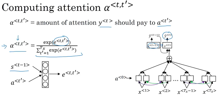
- \(\alpha^{<{t, t'}>}\) is amount of attention \(y^{<{t}>}\) should pay to \(a^{<{t'}>}\). In another word, to generate t-th output word how much weight pay to t’-th input word
- \(\displaystyle \sum_{ t }^{} {\alpha^{<{1, t'}>}} = 1\) all weights which used to generate 第一个的词的和等于1 (适用于每个词)
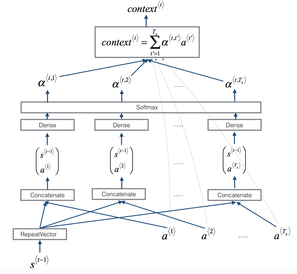
- \(\alpha^{<{t,t'}>} = \frac{ exp\left( e^{<{t,t'}>} \right) } { \sum_{t' = 1}^{T_x} { exp\left( e^{<{t,t'}>} \right) } }\) is softmax, ensure the sum of all weight equal 1
- to compute \(e^{<{t,t'}>}\), use small nerual network 如下图二 (通常只有一个hidden layer). input is
- \(s^{<{t-1}>}\) activation from previous time step in above RNN,
- \(a^{<{t'}>}\) the feature from timestep \(t'\).
- The intuition is to calculate attention for t from \(t'\), it depends on the what is hidden state activation from previous timestep and hidden stages RNN generating to look at French word feature
- Trust backprop and gradient descent to learn the right function
- Downside: take quadratic time to run this algorithm. total number of attention parameter is \(T_x\) x \(T_y\), where \(T_x\) total number of input and \(T_y\) the total number of output
- In machine translation application, neither input nor notput sentences not that long, so quadratic cost is acceptable
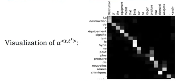
Visualization of attention weights: Attention weights tend to be high for corresponding input and output words. It suggests when generate a specific word in output is to pay attention to the correct words in the input
Speech recognition
- Audio Clip: horizontal axis is time, y-axis is air pressure detectde by microphone.
- Because human doesn’t process raw wave forms. Human ears measures the intensity of different frequency.
- A common step to preprocess audio data is to run raw audio clip and generate a spectrogram.
- x-axis is time, y-axis is frequencies, intensify of different colors shows the amount of energy(how loud the sound, different frequecies at different time?)
- Once Trend in Speech Recognition: speech recognition systems used to be built using phonemes(hand-engineer basic unit of cells)”de”, “kwik”… language can break down to these baisc unit of sound. Find that phonemes representations are no longer necessary
- need large dataset, academic dataset on speech recognition might be 3000 hrs. Best commerical system now train over 10000 hrs and sometimes over 100,000 hours of audio
Way to build Speech Recognition Model
Method 1: Attention Model: take different time frames of audio input and use attention model output transcript
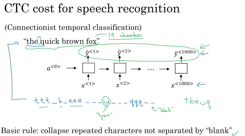
Method 2: CTC cost for speech recognition (CTC: connectionist temporal classification) Rule: collapse repeated characters not separated by “blank”
- Equal number of input x and output y and use bidirectional LSTM or bidirectional GRU in practice
- In speech recognition, input time steps are much bigger than output time steps(not equal);
- 比如10 seconds audio, feature come at 100 hertz so 100 samples每秒; 10 seconds audio clip has 1000 inputs, but output don’t have 1000 outputs for 1000 characters;
- CTC cost function is to collapse repeated characters not separated by blank. Then can have for example a thousand outputs by repeating characters to end up short transcrapt.
- _ : called special character, |_|: space character;
- e.g.
the_h_eee___|_|___qqq__end upthe|_|q - “The quick brown fox” only has 19 characters, CTC can allow have a thousand outputs by repeating charcters and inserting blank characters and still end up with 19 characters from 1000 outputs of values of Y
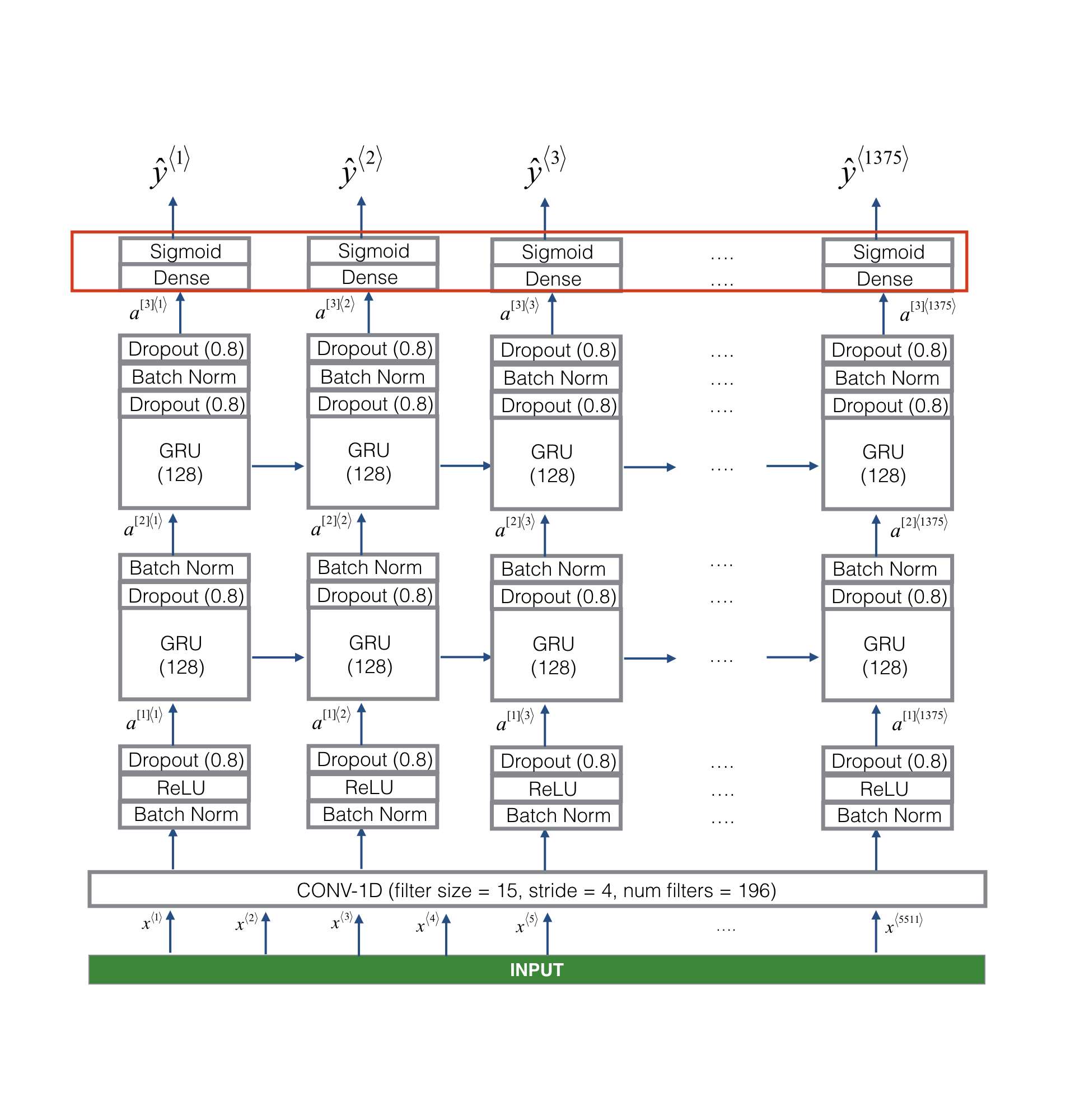
Trigger Word Detection
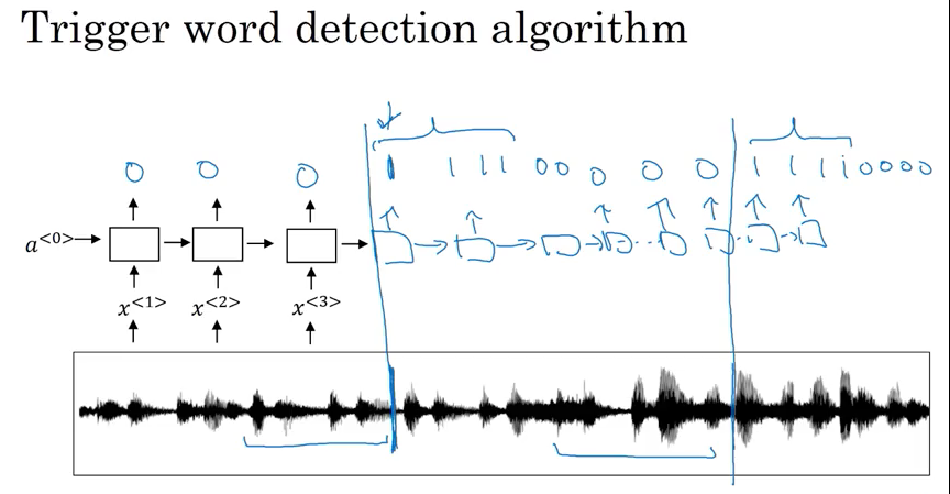
- 比如amazon echo; 用audio clip 计算spectrogram to generate features then pass to RNN; to define target label y when someone saying trigger word (小度小度,or hey Alexa) as 1, before and after trigger word set as 1
- could work. not work well, because it creates very imbalanced training set, a lots of zero than 1
- Solution: instead of setting single timestep as 1, make it 1 for a fixed period of time before revert back to 0(比如听到trigger word后, 接下来的几秒都设为1)
Paper Reference
- On the Properties of Neural Machine Translation: Encoder-Decoder Approaches, Cho, 2014: GRU Unit
- Empirical Evaluation of Gated Recurrent Neural Networks on Sequence Modeling, Chung, 2014: GRU Unit
- Long Short-Term Memory, hochreiter & schmidhuber, 1997: LSTM
- Visualizing Data using t-SNE, van der Maaten and Hinton, 2008: Visualize Word Embedding
- Linguistic Regularities in Continuous Space Word Representations, Mikolov, 2013: Cosine Similarity
- A Neural Probabilistic Language Model, Bengio, 2003: Neural Language Model fixed windows
- Efficient Estimation of Word Representations in Vector Space, Mikolov, 2013: Skip-grams
- Distributed Representations of Words and Phrases and their Compositionality, Mikolov, 2013: Negative Sampling
- GloVe: Global Vectors for Word Representation, Pennington, 2014: GloVe
- Man is to Computer Programmer as Woman is to Homemaker? Debiasing Word Embeddings, Bolukbasi, 2016: Debias word embeddings
- Sequence to Sequence Learning with Neural Networks, Sutskever, 2014: Machine Translation
- Learning Phrase Representations using RNN Encoder-Decoder for Statistical Machine Translation, Cho, 2014: Machine Translation
- Deep Captioning with Multimodal Recurrent Neural Networks (m-RNN), Mao, 2014: Image Captioning
- Show and Tell: A Neural Image Caption Generator, Vinyals, 2014: Image Captioning
- Deep Visual-Semantic Alignments for Generating Image Descriptions, Karpathy,, 2015: Image Captioning
- BLEU: a Method for Automatic Evaluation of Machine Translation, Papineni, 2002: BLeu Score
- Neural Machine Translation by Jointly Learning to Align and Translate: Attention Model
- Show, Attend and Tell: Neural Image Caption Generation with Visual Attention, Xu, 2015: Attention Model Application: look at the picture and pay attention only to parts of picture at a time while writing a caption for a picture
- Connectionist Temporal Classification: Labelling Unsegmented Sequence Data with Recurrent Neural Networks, Graves, 2006: CTC cost for speech recognition