1 Convolution Neural Networks
Computer Vision Challenge: the input can be really big, e.g if a image 1000*1000 pixel,Each pixel is controlled by three rgb channel,image input is 1000*1000*3. Input is 3 million, and the first hidden layer(e.g. fully-connected network) has 1000 units, the weight will be (1000, 3 Million), 3 billion parameters. It is difficult to get enough data to avoid overfitting and the computational requirement and memory requirement to train is infeasible/expensive
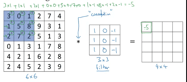
Edge Detection
Vertical Edge Detection
convolve image by filter (Kernel)
e.g. Vertical edge detection
Why above filter works for vertical detection? e.g. the image(left matrix), left half give brigther pixel intensive and right half give darker pixel intensive values.
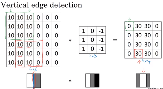
Above detected edge (value 30, 2 columns) seems very thick, because we use only small iamges. If you are using 1000 by 1000 image rather than 6 and 6, it does pretty good job
Inituition: vertical edge detection, since example filter use 3 by 3 region where bright pixels on the left and dark pixels on the right (don’t care about what’s in middle in filter)
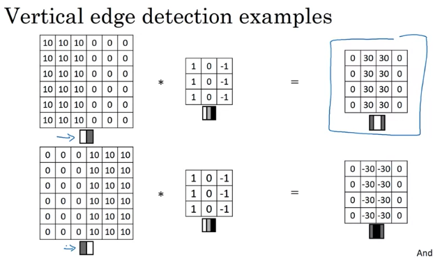
-30 example, could take absolute values of output matrix. But this filter does make the difference between light to dark vs dark to light
Horizontal Edge Detection
light on top and dark on the bottom row
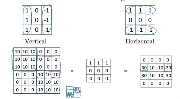
Above example:
- 30 is the edge that light on top and dark on bottom
- -30 is the edge that dark on top and light on bottom.
- -10 reflect that parts of positive edge on the left and parts of negative edge on the right, gives some intermediate value. But if a image is 1000x1000, won’t see these transitions regions of 10s. The intermediate values would be quite small relative to the size of iamge.
# Conv-forward
tf.nn.conv2d #TensorFlow
Conv2D       #Keras
Filter
Sobel filter: advantage: put more weight in the middle(2, -2), make it a little bit more robust \(\begin{bmatrix} 1 & 0 & -1 \\ 2 & 0 & -2 \\ 1 & 0 & -1 \\ \end{bmatrix}\)
Scharr filter:
\[\begin{bmatrix} 3 & 0 & -3 \\ 10 & 0 & -10 \\ 3 & 0 & -3 \\ \end{bmatrix}\]can filp above 90 degree to get horizontal edge detection
也许不用hand pick those number,让computer 自己学 \(\begin{bmatrix} w_1 & w_2 & w_3 \\ w_4 & w_5 & w_6 \\ w_7 & w_8 & w_9 \\ \end{bmatrix}\) The goal: give a image, convolve it with 3x3 filter, that gives a good edge detector. It may learn something even better than hand coded filter. 通过neural network backprop,也许不是vertical的,也许是 detect 45度的,70度的
Padding
if image is n x n the filter is f x f and the output is \(n-f+1 \times n-f+1\)
Downside of filter:
- Image will shrink if performing convolution neural networks (to (n-f+1)*(n-f+1) ) 2. Corner pixel only be used once(e.g. upper-left, upper-right), but middle pixel used by multiple times, throw away a lot of information near the edge of the image
Solution: pad the image by additional border. e.g. 6 x 6 pad to 8 x 8, filter is 3 x 3, then the output is 6 x 6
Denote p = padding amount, above example 6 x 6 to 8 x 8, p = 1, padding on top, left, bottom, right by 1
- Valid convolutions: no padding:
n x n * f x f = (n-f+1) x (n-f+1) - Same convolutions: Pad so that output size is the same as the input size.
(n+2p - f+1) x (n+2p - f+1) = n x n=>p = (f-1)/2. so when filter is3x3,p=1, when fitler is5x5,p=2
Filter size f usually be odd
number, the convention in computer vision. If f is even, you will come up asymmetrix padding, Besides, when have odd number of padding, you will have a central position in the middle for the filter.
Strided Convolution
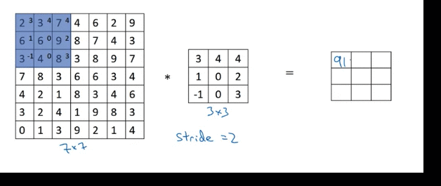
round down to the nearest integer if fraction is not integer (Floor). For above example, (7 + 0 - 3)/2 + 1 = 3
If after padding, the the filter box hangs outside of image, don’t do that computation
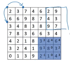
Convolutional Operation
The operation done before is called cross-correlation instead of convolution operation.
By convention in machine learning, 通常忽略 flipping operation. The operation done before better called cross-correlation, but most of deep learning literature called it convolutional operater(without flip)
The convolution before product and summing is to flip filter horizontal and vertically. Then use flipped filter to compute element wise product and summation e.g.
\[\begin{bmatrix} 3 & 4 & 5 \\ 1 & 0 & 2 \\ -1 & 9 & 7 \\ \end{bmatrix}\]to
\[\begin{bmatrix} 7 & 9 & -1 \\ 2 & 0 & 1 \\ 5 & 4 & 3 \\ \end{bmatrix}\]Convolution satisfy associativity: A convolve B convolve C equal to A convolve (B convolve C)
\[\left( A * B \right) * C = A * \left( B * C \right)\]Convolutions Over Volume
input is 6 x 6 x 3 where 3 is the color channel(red, green, blue), the filter is 3 x 3 x 3. Denote first demension is height, second demension is width, third dimension is channel(in literature, some people called it depth). The number of channel in image must match the channel of the filter
Below example, filter size is 3 x 3 x 3, element wise product for image and filter, for the first channel, second channel, third channel one by one. then add those 27 number together as output
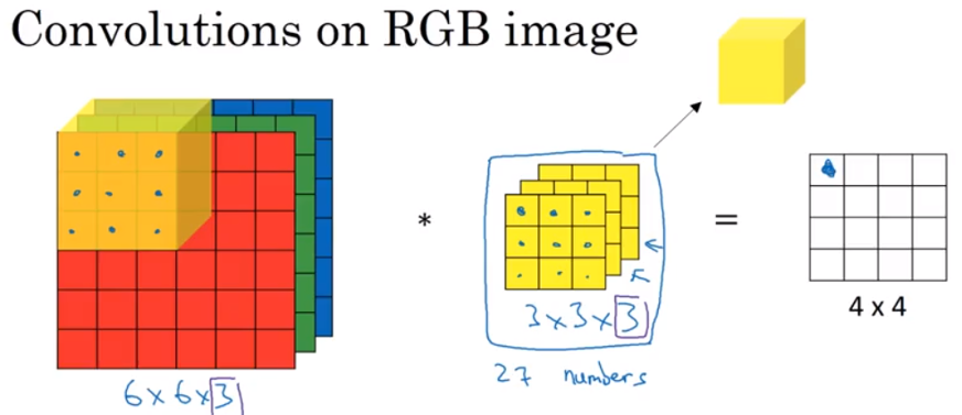
e,g1, if you want to detect vertical edges in the red channel,
\[\underbrace{\begin{bmatrix} 1 & 0 & -1 \\ 1 & 0 & -1 \\ 1 & 0 & -1 \\ \end{bmatrix}}_{red}, \underbrace{\begin{bmatrix} 0 & 0 & 0 \\ 0 & 0 & 0 \\ 0 & 0 & 0 \\ \end{bmatrix}}_{green}, \underbrace{\begin{bmatrix} 0 & 0 & 0 \\ 0 & 0 & 0 \\ 0 & 0 & 0 \\ \end{bmatrix}}_{blue},\]e.g2 If want to detect edges, then could use
\[\underbrace{\begin{bmatrix} 1 & 0 & -1 \\ 1 & 0 & -1 \\ 1 & 0 & -1 \\ \end{bmatrix}}_{red}, \underbrace{\begin{bmatrix} 1 & 0 & -1 \\ 1 & 0 & -1 \\ 1 & 0 & -1 \\ \end{bmatrix}}_{green}, \underbrace{\begin{bmatrix} 1 & 0 & -1 \\ 1 & 0 & -1 \\ 1 & 0 & -1 \\ \end{bmatrix}}_{blue},\]If want to detect both horizontal and vertical edges, use multiple filters (first filter to detect horizontal and second filter to detect vertifal). Then the first output at the front, and second output at back
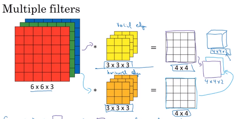
Summary: n x n x n_c(the number of channel) * f x f x n_c = (n – f + 1) x (n – f + 1) x n_c’ (n_c’ is the number of filter we used), assumed stride one and no padding
Convolutional Network
After convolve using filter, add a real number bias to every number in the output then apply non-linearity (e.g. Relu) (一个filter 一个bias)
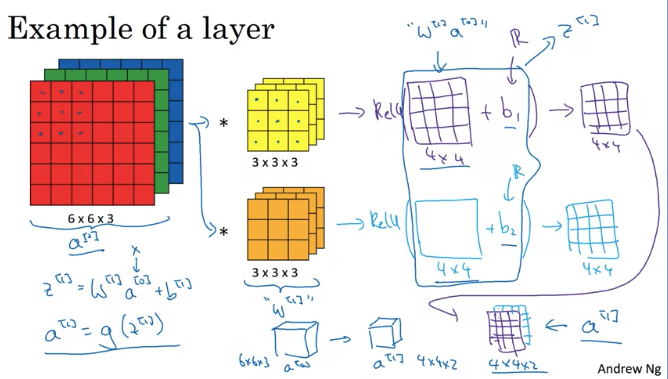
Notice: filter is the \(W\)
Q: if have 10 filters that are `3x3x31 in one leayr of a neural network, how many parameters that layer have
A: each filter has 3x3x3 = 27 filter plus one bias, so 10 filter has 28x10 = 280 parameters
Notation
if layer l is a convolution layer:
\[f^{\left[ l \right]} = \text{filter size}\] \[p^{\left[ l \right]} = \text{padding}\] \[s^{\left[ l \right]} = \text{stride}\] \[n_c^{\left[ l \right]} = \text{number of filters}\]Input: \(n_c\) is the number of, use superscript l-1 because that’s the activation from previous layer, H and W denotes height and width
\[\text{Input: }n_H^{\left[ l-1 \right]} \times n_W^{\left[ l-1 \right]} \times n_c^{\left[ l - 1 \right]}\] \[\text{Output: }n_H^{\left[ l \right]} \times n_W^{\left[ l \right]} \times n_c^{\left[ l \right]}\] \[\text{where the height and width: } n^{\left[ l \right]}= \lfloor \frac{n^{\left[ l-1 \right]} + 2p^{\left[ l \right]} -f^{\left[ l \right]}}{s^{\left[ l \right]}} + 1 \rfloor\] \[\text{Each filter is } f^{\left[ l \right]} \times f^{\left[ l \right]} \times n_c^{\left[ l-1 \right]}\] \[\text{where }n_c^{\left[ l-1 \right]} \text{ last layer's number of channel}\] \[\text{Activations: } a^{\left[ l \right]} -> n_H^{\left[ l \right]} \times n_W^{\left[ l \right]} \times n_c^{\left[ l \right]} \text{or some write } a^{\left[ l \right]} -> n_c^{\left[ l \right]} \times n_H^{\left[ l \right]} \times n_W^{\left[ l \right]}\] \[\text{Weights}: f^{\left[ l \right]} \times f^{\left[ l \right]} \times n_c^{\left[ l-1 \right]} \times n_c^{\left[ l \right]}\] \[\text{bias: } n_c^{\left[ l-1 \right]}, \text{in program, deminsion write: } \left(1,1,1,n_c^{\left[ l \right]} \right)\]If using batch gradient descent or mini batch gradient descent:
\[\text{Activations: } A^{\left[ l \right]} -> m \times n_H^{\left[ l \right]} \times n_W^{\left[ l \right]} \times n_c^{\left[ l \right]}, \text{m examples}\]An example of ConvNet
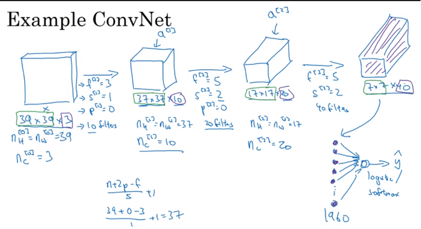
Input : 39 x 39 x 3 image
role out ` 7 x7 x 40 = 1960 ` to unroll 1960 units into a long vector and feed into a logistic regression unit or a softmax unit
Lots of work in designing convolutional neural net is selecting hyparameters like deciding what’s total size? filter size? padding? how many filter are use?
Typically, start with a large image, then height and width will stay the same for a while and gradually trend down as go deeper in the neural network whereas the number of channel general increase
Pooling Layer
Pooling: reduce the size of the representation to speed computation as well as make some of the features that detects a bit more robust.
Max Pooling: Intuition: If these features detected anywhere in this filter, then keep a high number. If feature not detected, then maybe this feature doesn’t exist in this quadrant. People Found a lot of experiences to work well.
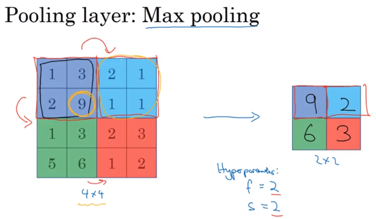
Property: Above example, hyparameter filter size = 2(because take 2 by 2 region) and stride = 2, but has no parameter to learn. Once fix f and s, just a fixed computation and gradient descent doesn’t change anything
If have 3D input, max pooling is done independently on each of channel one by one and stack output together(每个channel分开max pooling, 然后stack together)
Average Pooling: Instead of taking max of each filter, take the average of each filter. not used often compared Max Pooling. One exception: Very deep neural network, you might use average pooling to collapse representation. e.g. (7 x 7 x 1000 to 1 x 1 x 1000)
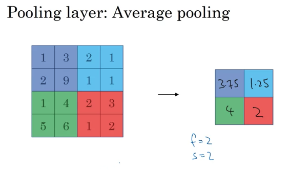
Max or average pooling. 或者有时候 (very very rare ) add padding , most of time max pooling p = 0, no parameter to learn!
Common choice of f = 2, s = 2, has the effect of shrinking the height and with of representation by factor of two. Some use f = 3, s = 2
The formula still works. Since pooling applies each of channel independently, the number of input channel match the number of output channel
\[n_H \times n_W \times n_c = \lfloor \frac{n + 2p -f}{s} + 1 \rfloor \times \lfloor \frac{n + 2p -f }{s} + 1\rfloor \times n_c\]CNN Example
example inspired by LeNet-5
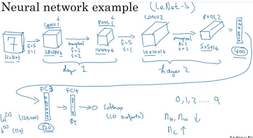
| Activation shape | Activation Size | num of parameters | |
|---|---|---|---|
| Input | (32, 32,3) | 3072 | 0 |
| CONV1(f=5, s = 1) | (28,28,8) | 6272 | 608 ((5*5*3+1)*8) |
| POOL1 | (14,14,8) | 1568 | 0 |
| CONV2(f=5, s=1) | (10,10,16) | 1600 | 3216 (5*5*8+1)*16 |
| POOL2 | (5,5,16) | 400 | 0 |
| FC3 | (120, 1) | 120 | 48120 400*120+120(120 bias) |
| FC4 | (84, 1) | 84 | 10164 120*84 + 84 |
| Softmax | (10, 1) | 10 | 850 |
When report number of layer, people usually report the number of layers that have weight, that have parameters. Beacuse pooling layer has no weights and no parameters only has hyperparameters, so put ConV and pooling layer together in convention.
Guideline: not to invent your own hyperparameter, but look into literature to see what hyper parameters you work for others, just choose a architecture that works well for others and there is a chance that works well for you as well.
Common pattern one or more conv layers followed by a pooling layer and in the end have a few fully connected layers then followed by a softmax
Notice:
- pooling layer has no parameters
- Conv layer tend to have a few parameters and lots of parameters tend to be in the fully connected layer
- Activation size tend of go down gradually as go deeper in the neural network. If drop too quickly, not great for performance as well
Why Convolutions
Two main advantage of using Conv layer instead of fully connected layer(parameter sharing & sparsity of connections : 因为parameter 少了,allowed to train a smaller training set and less proned to overfitting).
- parameter sharing: A feature detector (such as vertical edge detector) that’s useful in one part of the image is probably useful in another part of the image
- e.g. apply 3 by 3 filter on the top-left of the image and apply the same filter on top-right of the image.
- True for low-level features(edges and blobs) like edges as well as high-level features(objects) like detecting the eye that indicates a face or a cat
- sparsity of connections : In each layer, each output value depends only on a small number of inputs. 比如filter 是
3*3, output 第1行1个只取决于 input 的top left3*3parameter,不取决于 第一行第四个或者第五个值 - Convolution neural network aslo very good at capturing translation invariance(即使原来图片发生一点点位移,还是原来feature) e.g 比如一只猫shift couple of pixels to right 仍是猫. And convolutional structure helps that shifted a few pixels should result pretty similar feature. Apply the same filter on the image helps to be more robust to caputre the desirable property of translation invariance
e.g.
\[\require{AMScd} \begin{CD} \underbrace{\text{Image 32 x 32 x 3}}_{3072} @>{\text{f = 5, 6 filters}}>> \underbrace{\text{28 x 28 x 6} }_{4074} \end{CD}\]- A fully-connected layer: the number of parameters is
3072 x 4074 = 14 million - Convolutional layer:
(5 x 5 x 3 + 1 ) x 6 = 456parameters
Cost function: Use gradient descent or gradient descent momentum, RMSProp or Adams to optimize parameters to reduce J
\[J = \frac{1}{m} \sum_{i=1}^m L\left(\hat y^{\left(i \right)}, y^{\left(i \right)}\right),\text{where }, \hat y \text{ is the predicted label and y is true label}\]Backprop
use l denote layer, f denote filter size and assume stride = 0 and only 1 filter(So, if input is 9x9x3 and filter is 3x3x3 output will be 7x7), A denote the activation, \(n_c\) denotes the number of channel. H,W denotes heights and width
So
\[\begin{align} \frac{\partial L}{\partial W_{i,j,k}^l} &= \sum_{m=0}^{H} \sum_{n=0}^{W} \frac{\partial L}{\partial Z_{m,n}^l}\frac{\partial Z_{m,n}^l }{\partial W_{i,j,k}^l} \\ &= \sum_{m=0}^{H} \sum_{n=0}^{W} \frac{\partial L}{\partial Z_{m,n}^l} A_{i+m,j+n,k}^{l-1} \end{align}\]In vectorized expression
\[dw \left[:,:,: \right] += A^{l-1}\left[m:m+f, n:n+f,: \right] * dz\left[m, n\right]\]Point Z[m,n] convolve from \(A^{l-1}\left[m:m+f, n:n+f,: \right]\) and the whole filter
In vectorized expression, db size is 1 x 1
In vectorized expression
2. Classic Networks
LeNet-5
Last year is softmax layer although back then, LeNet-5 used a different classifier at the output which is useless today.
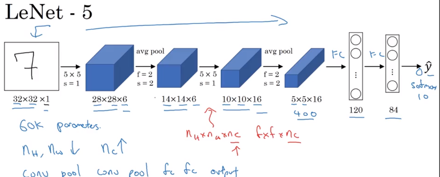
Above model has 60k parameters. Today, often see a network with 10 million to 100 million parameters. When you go deeper with your network, the height and weight tend to go down and the number of channel tend to increase.
Pattern often used today:
\[\require{AMScd} \begin{CD} \text{one or more Conv Layer} @>>> \text{Pooling Layer} @>>> \text{one or more Conv Layer} @>>> \text{Pooling Layer} \\ @. @. @. @VVV \\ @. \text{output} @<<< \text{fully-connected layer} @<<< \text{fully-connected layer} \end{CD}\](Optional): In paper, use sigmoid and tanh in the paper (no ReLu used at that time). Besides, in paper, use sigmoid non-linearity after the pooling layer(not used today)
Alexnet
Alexnet has a lot of similarity to Lenet but it was much bigger. Lenet has around 60 thousand parameters whereas Alexnet has 60 million parameters.
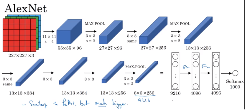
- Compared to LeNet, the fact that they could take similar building block, but a lot more hidden units and training on a lot of more data to allow it to have a remarkable performance
- Another aspects make it much better than LeNet is using Relu activation function
- had a complicated way of training on two GPUs. A lot of ConV and pooling layer split across two different GPUs and a thoughtful way for when two GPUs communicate with each others.
- Local Response Normalization(not use too much): 方法: 一个block 是
13*13*256,比如把第一维是5, 第二维是6的上所有的256 的数,normalize 这256个数据- Motivation: maybe you don’t want for each position in 13 by 13 image,you don’t want too many neurons with a very high activation. But subsequently, some researcher 发现local response normalization less important(Andrew Ng doesn’t use it)
VGG-16
Motivation: instead of having so many hyperparameters, use a much simpler network where focus on just having ConV layers that are just 3 by 3 filters with stride one, and always use the same padding. And make all your max pulling layers 2 by 2 with stride of two; it simplify this neural network architectures.
Downside: large netowrk in terms of the number of parameters you train
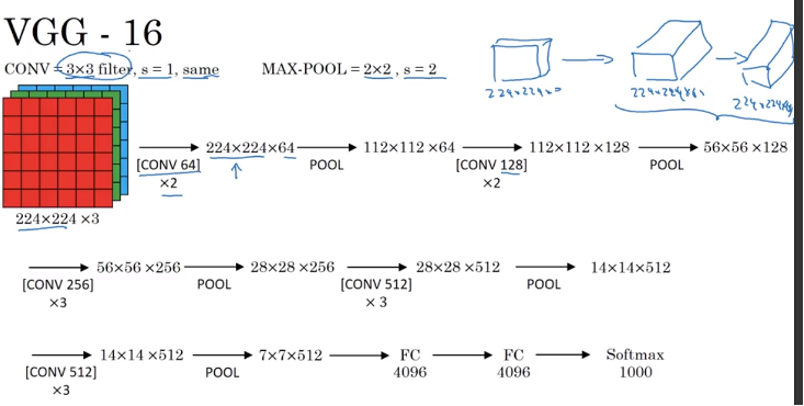
- VGG-16: 16 layers have weights
- This network has 138 million parameters, large network
- The architecture is really quite uniform, a few ConV layers followed by a polling layer whereas the pooling layers reduce the height and weight. Number of channel from 64 到128, 到256,到512(512 is big enough, not need to double), roughly doubling on every step or doubling through every stack of ConV layers is another principle used to desgin the architecture of this network
Some literature mention VGG-19. It’s even bigger version of this network.
3. ResNets
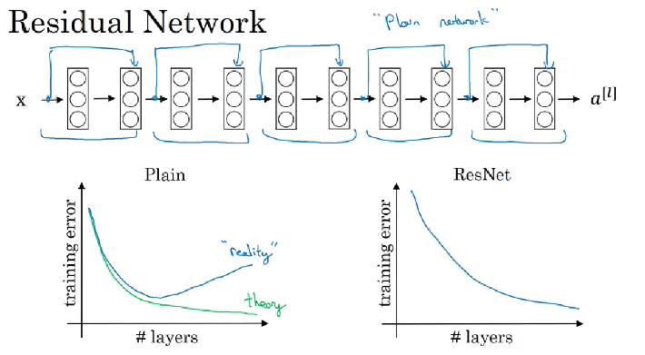
ResNets: Very deep neural Networks are difficult to train because gradient vanishing/exploding problem. ResNets enables you to train very very deep networks (sometimes even over 100 hundred layers)
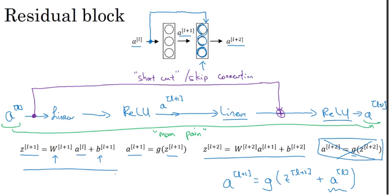
Residual Blocks : take \(a^{\left[l \right]}\) fast foward it, copy it to much further into the neural networks,inject after the linear part but before perform nonlinear function (ReLu): called it Shortcut(skip connection) using
Residual blocks allow you train much deeper neural network. The way to build ResNet is by taking many of these residual blocks and stacking them together to form a deep network
if use optimization algorithm such as gradient descent to train a plain neural network, without extra shortcuts or skip connections, training error like below graph. But in reality your training error get worse(train error first decrease then increase) if you pick a network that’s too deep.
For ResNet is that even as the number of layers gets deeper, having the performance of training error keeping going down, even train over a hundred of layers. It helps with the vanishing and exploding problems. It allows train much deeper neural networks without appreciable loss in performance
Why work?
For example, if have a network below, we have Relu and assume a is bigger than or equal to 0.
\[\require{AMScd} \begin{CD} @. @. @>{\text{short cut}}>> --> @>{\text{short cut}}>> a^{\left[l \right]} \\ @. @. @AAA @. @VVV \\ x @>>> BigNN @>>> a^{\left[l \right]} @>>> layer1 @>>> layer2 @>>> a^{\left[l+2 \right]} \end{CD}\]then
\[\begin{align} a^{\left[l + 2 \right]} &= g\left( z^{\left[l + 2 \right]} + a^{\left[l \right]} \right) \\ &= g\left( w^{\left[l + 2 \right]}a^{\left[l + 1 \right]} + b^{\left[l + 2 \right]} + a^{\left[l \right]} \right) \end{align}\]If you use L2 regularization to shrink \(w^{\left[l + 2 \right]}\) , then if you apply weight to b it will also shrink weight to b although in practice don’t apply regularization weight to b, if \(w^{\left[l + 2 \right]} =\) and \(b^{\left[l + 2 \right]} = 0\)
\[a^{\left[l + 2 \right]} = g\left( a^{\left[l \right]} \right) = a^{\left[l \right]}\]Note: we assume \(z^{\left[l + 2 \right]}\) and \(a^{\left[l \right]}\) have the same dimension. Use the same convolution
But if they don’t have the same dimension, add \(W_s\), e.g. \(z^{\left[l + 2 \right]}\) 256 维, \(a^{\left[l \right]}\) 128 维, then \(W_S\) is 256 by 128. \(W_S\) could a parameter to learn or a fixed matrix that just implement zero paddings (padding 128 to 256)
\[a^{\left[l + 2 \right]} = g\left( z^{\left[l + 2 \right]} + W_Sa^{\left[l \right]} \right)\]It shows the because of skip connection, it’s so easy for residual networks to learn identity function, guarantee adding residual blocks doesn’t hurt neural network performance and gradient descent can improve the solution , it’s easy to get \(a^{\left[l + 2\right]}\) equal to \(a^{\left[l \right]}\). Hidden units if actually learn something useful then can do even better than learning the identity function
In plain network without Residual Network, when you make the network deeper and deeper, it is very difficult for it to choose parameters that learn even the identity function, which a lot of layer end-up worse.
Resnet on Image
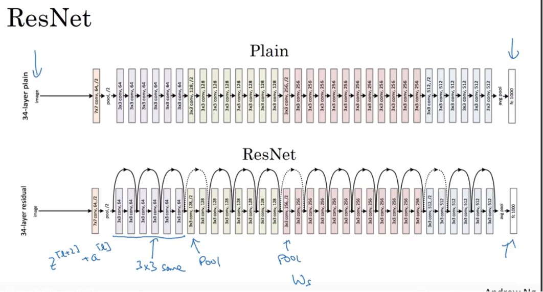
- lots 3 by 3 convolutions. And most of them are 3 by 3(filter size) same convolution instead of fully-connected layer . That’s why \(z^{\left[l + 2 \right]} + a^{\left[l \right]}\) make senses
- After pooling layer, need to adjust dimension, liked discussed above by \(W_S\)
- In the end, have a fully connected layer that makes a prediction using a softmax
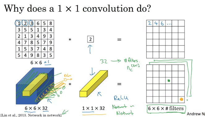
3. 1x1 Convolution
sometimes 1x1 Convolution called Network in Network
What does it do in the below example: look at each of the 36 different positions, and take the element-wise product between 32 numbers on the input (same height and same width) and 32 numbers in the filter, add together(summation) then apply Relu non-linearity(32 -> 1 number).
One way to think of 1 by 1 convolution is bsically having a fully connected neural network that applies to each of 36 different position
Use of 1x1 Convolution
- Shrink the number of channel(save computation): usually pooling is used to shrink height and weight. 而1*1 convolution 是 比如input 是
28*28*192,1*1dimension convolution 是1*1*19232 filters,output is28*28*32which allow shrink \(n_c\) as well whereas Pooling layer only shrink \(n_H\) and \(n_W\) - If want to keep the number of Channel, 1 by 1 convolution add linearity to allow to learn more complex function of your network by adding this layer , 接着上面例子, filter size is
1x1x192and have 192 filters, output will be28*28*192(28*28*192 -> 28*28*192)
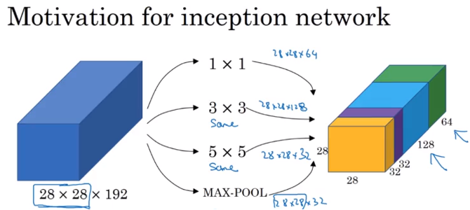
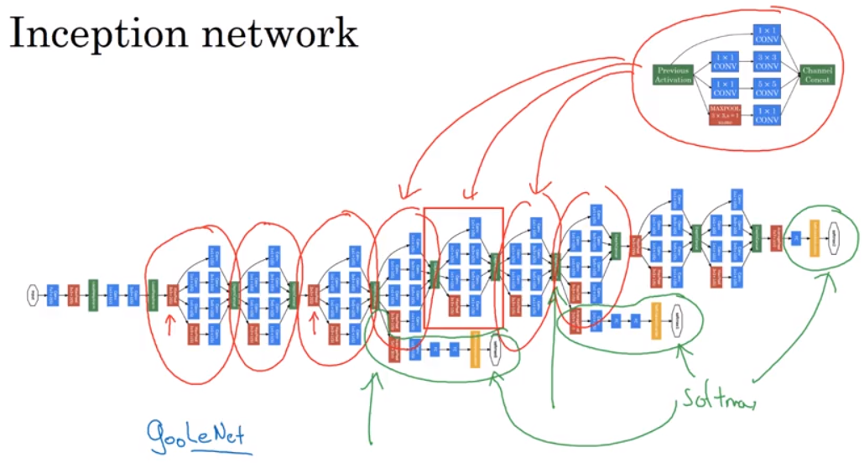
4. Inception Network
Instead of choosing to filter size, or choose convolutional layer or pooling layer, let use them all together, stack(concatenate) all output \ together
e.g. image input is 28 x 28 x 192,
- use 64 filters with size
1 x 1 x 192, get28 x 28 x 64 - use 128 filters with size
3 x 3 x 192, same convolution, get28 x 28 x 128 - use 32 filters with size
5 x 5 x 192, same convolution, get28 x 28 x 32 - max pooling and 1 by 1 convolution, get
28 x 28 x 32, need padding to get the same height and width - Stack previous output together
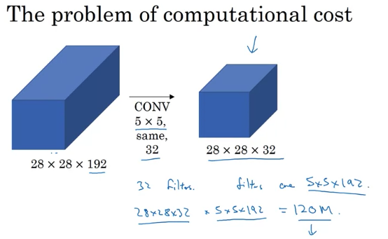
A problem: Computational Cost
e.g. 32 filters with each size 5 x 5 x 192, output size is 28 x 28 x 32, each output is needed to calculate 5 x 5 x 192 multiplications. Total number of multiplications is 28 x 28 x 32 x 5 x 5 x 192 = 120 million, expensive operation. Could use 1 by 1 convolution to reduce the computational costs by a factor of 10
Use 1 by 1 convolution, can see output dimension is the same. First shrink to much smaller intermediate volume 28 x 28 x 16 called bottleneck layer
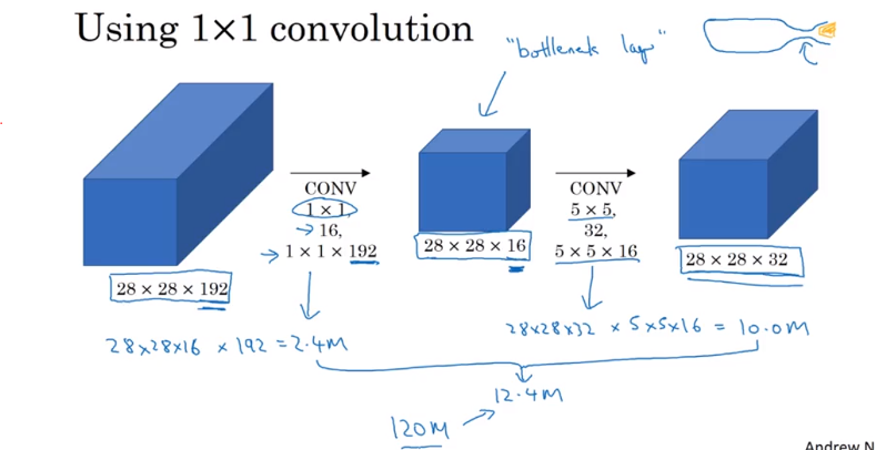
Computation Cost: Cost of first convolutional layer 28 x 28 x 16 x 1 x 1 x 192 = 2.4 million. 28 x 28 x 32 x 5 x 5 x 16 = 10 million. total is 12.4 million << 120 million
- Apply 64 filters of 1 by 1 convolution, get
28 x 28 x 64output - Apply 96 filters of 1 by 1 convolution, then apply 128
3 x 3filters to get28 x 28 x 128output - Apply 16 filters of 1 by 1 convolution, then apply 32
5 x 5filters to get28 x 28 x 32output - For above example pooling,in order to concatenate all of outputs at the end, use the same type of padding for pooling. The output will be
28 x 28 x 192. Then apply one more 1 by 1 convolutional layer to shrink the number of channel to28 x 28 x 32 - In the end, channel concatenation
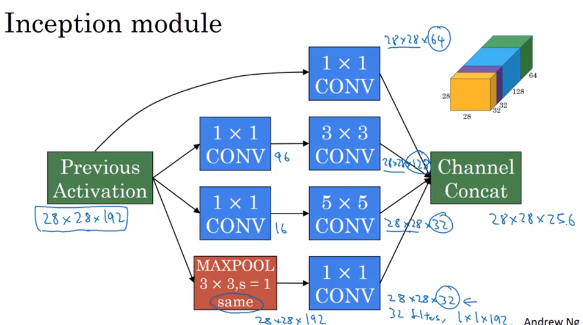
What the inception network does is to put all inception block together. 下面的inception network 是多个上面的repeated inception block stack在一起. 红色小箭头是max pooling to change the height and width
Inception network 有side branch,takes a hidden layer to pass through a few fully-connected layer, then has a softmax to make prediction, It is said even in intermediate(hidden) layer 加上几层用softmax, not so bad to predict outcomes. It also has regularization effect, prevent network overfitting (避免训练network too deep)
5. Advices for ConvNets
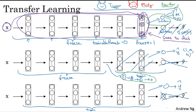
Transfer Learning
Sometimes, training takes several weeks and might take many GPU. Can download open source weight that took someone else many weeks or months as a good initialization for your own neural network.
When don’t have enough training data:
download Github open-source implementation and weight, then get rid of softmax layer and create your own softmax unit. Take early stage layers and parameters as frozon. And train the parameters associated with your softmax layer. Then might get good performance even with a small dataset(只train softmax layer)
Some deep learning framework can let you specify whether to train parameter or freeze parameters.
Trick: because of all of early layers are frozon, Use some fixed function to take a image to the activation in the layer which you begin to train. Can pre-compute that layer(image 和所有froozen layer 到开始训练的layer) and save to disk. Then train a shallow softmax model to make a prediction
Advantage: don’t need to recompute the activations everytimes
If have a large training set:
- freeze a fewer layer, then train latter layers and create the your own output unit.
- Or delete these latter layers and just use your own new hidden units and your own softmax output.
- Or train some other size neural networks(different size of hidden layers) that comprise last layer of your own softmax output
- If have lots of data, take whole things as initialization(to replace random initialization) and train the whole network and update all the weights of all the layers of the network by gradient descent
When having more data, the number of layers freeze could be smaller and the number of layers trained could be greater.
Transfer learning is something should always do unless have exceptionally large data and very large computation budge
Data Augmentation
- Mirroring: 比如一个猫的图片左右颠倒下 and Mirroring preserves what is in the picture
- Random Cropping: 随机选取图片的一部分剪切下来,当做新的,random cropping isn’t the perfect way for data augmentation. In practice, it works well.
- Some other method: rotation, shearing(正方形变平行四边形), local warping: no harm with trying of all these things. But in practice, they seem to be used a bit less. perhaps because of complexity
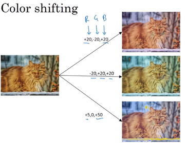
- Color shifting: 比如red 增加 20, green 减小20, 蓝色增加20. In practice, R,G, and B are drawn from some probability distribution
- Motivation: maybe sunlight might a little bit yellow that could easily change the color of the image but the indentity of the content (y) should stay the same
- Introduce color shifting, make learning algorithm more robust to change in colors of image
One of the ways to implement color distortion algorithm: PCA color Augmentation
What PCA do: 比如 image mainly has red and blue tints, and very little green. PCA color Augmentation will add / subtract a lot for red and blue and very little green so that keeps the overall color the tint the same.
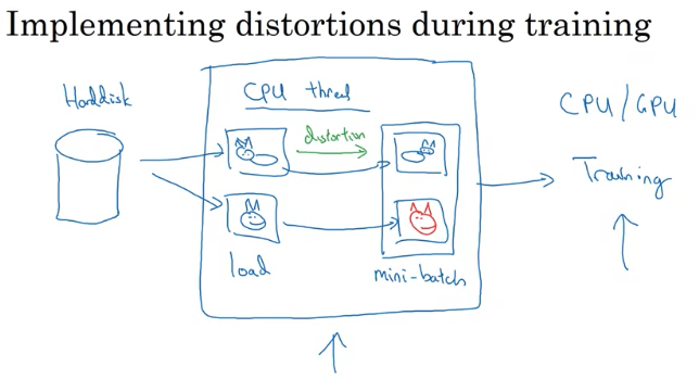
Implementing distortions during training:
if you have large training set:
- have a CPU thread that is constantly loading images of your hard disk, then implement distortion (random cropping, color shifting, or mirroring) to form a batch or mini-batches of data
- Then batch / mini-batches are constantly passed to some other thread or process for training(CPU or increasingly GPU if have a large neural network to train)
- Above two thread can run in parallel
Data augmentation 有时候还可以 有hyperparameter 去tune,比如 how much color shifting do you implement and exactly what parameters you use for random cropping.(If you think someone else doesn’t not captured more in variances in their implementation, it might be reasonable to use hyperparameters yourself)
State of Computer Vision
Image recognition 是给图片告诉是猫还是狗,object detection 是给你图片where in picture 有障碍物(autonomous driving)we tend to have less data for objection detection than for image recognition (because of the cost of getting bounding box to label is more expensive than label the objects)
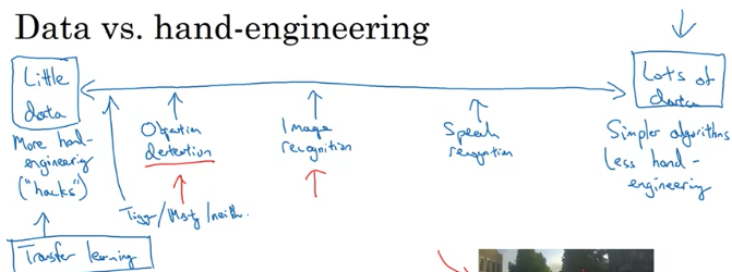
- When have lots of data, Can have a giant neural networks, use simple algorithms as well as less hand-engineering. Less needing to carefully desgin features for the problem to learn whatever to learn if having lots of data
- When don’t have too much data, more hand-engineering. Hand-engineering is the best way to get good performance when has less data.
Two sources of knowledge:
- Label data (x, y)
- Hand engineered features/network architecture/other components
Computer Vision is trying to learn really a complex function. We don’t have enough data for computer vision. Even datasets are getting bigger and bigger, often we don’t have as much data as we need. That’s why computer vision relied more on hand-engineering. That’s way computer vision has developed complex architectures becaue of the absence of more data. 即使最近data increase dramatically, results in a significant reduction in amount f hand-engineering. 但是still lots of hand-engineering of network architectures in computer vision compared to other disciplines.
When don’t have enough data, hand-engineering is very diffcult, skillful task that requires a lot of insight. If have lots of data, wouldn’t spend time hand-engineering, would spend time to build up the learning system.
Tips for doing well on benchmarks:
- Ensembling: Train and Run several neural network independently(3-15 network) and average their output (average \(\hat y\), not average weight which won’t work) 因为速度会降很多倍,所以用它来win in competition not use in actual production to serve customer 同时ensembling 因为是run 了很多network,会用掉很多memory to keep all these network around (Computational expensive)
- Multi-crop at test time: Run classifier on multiple versions of test image and average results. Multi-crop is applying data agumentation to your test image. It might get a little bit better performance in a production system.
- 一张图片随机选取其中好几个部分作为test sample,每一个sample运行network through classifier,average results
Andrew Ng: 以上方法是research 中提到的,不建议用in production or a system that deploy in an actual application
建议:
- Use open-source code implementations if possible
- Use architectures of networks published in the literature
- use pretrained models and fine-tune on your dataset to get faster on an application(transfer learning: someone else may train a model on half dozen GPU and over a million images)
6. Object Detection
Object Localization
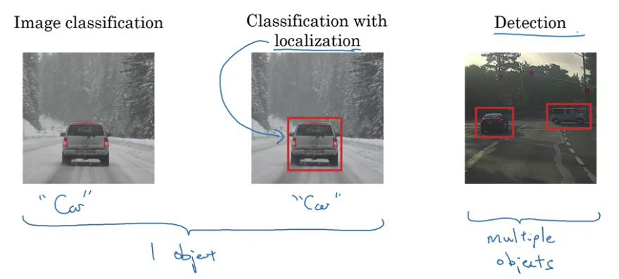
- Image classification: recognize it’s a car
- Classification with localization: algorithm not only label the image as a car but aslo responsible for putting a bounding box. Localization 表示 where in the picture care you’ve detected. Usually one big object in the middle of the image that trying to recognize
- Detection: multiple objects in the picture, detect them all and localized them all. Or even multiple objects of different categories within a single image.
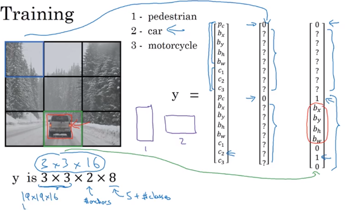
For Autonomous driving, softmax may predict four categories: pedestrain, car, motorcycle, or backaground.
Localization: Change your neural networks to have a few more output units that output a bounding box.
- Use upper left of the image as (0,0) and lower-right as (1,1). Specifying the bounding box, red rectangle reqires specifying the midpoint (\(b_x, b_y\)), height and widths of the rounding box (\(b_h, b_w\)). \(b_h, b_w\) bounding box的长宽 占整个图片的多少,而不是起始点的坐标
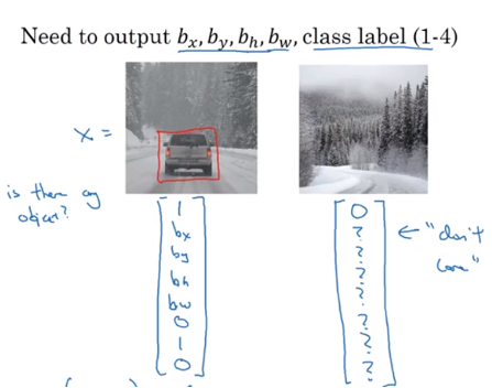
- So training set not only contain class label and also contain 4 additional numbers (\(b_x, b_y, b_h, b_w\))
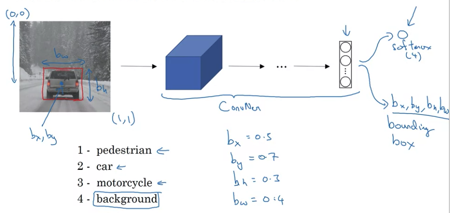
- \(P_c = 1\) if object is predestrian, car, else motorcycle; \(P_c = 0\) if background. \(P_c\) is the probability that one of the classes you’re trying to detect is there
- \(c_1, c_2, c_3\) tell if \(P_c = 1\) tell the class if pedestrian, car, or motorcycle.
- if \(P_c = 0\), don’t care following output in y
Loss Function
\[L\left(\hat y, y \right) = \left\{ \begin{array}{ll} \left( \hat y_1 - y_1 \right)^2 + \left( \hat y_2 - y_2 \right)^2 + \cdots + \left( \hat y_8 - y_8 \right)^2 & \text{for y = 1} \\ \left( \hat y_1 - y_1 \right)^2 & \text{for y = 0}\\ \end{array} \right.\]Squared error for all outputs is simplified description. In practice, use loglikelihood loss for \(c_1, c_2, c_3\) (the softmax output); squared error for bounding box cordinates (\(b_x, b_y, b_h, b_w\)) ;\(p_c\) could use logistic regression loss. Although use squared error, it works ok.
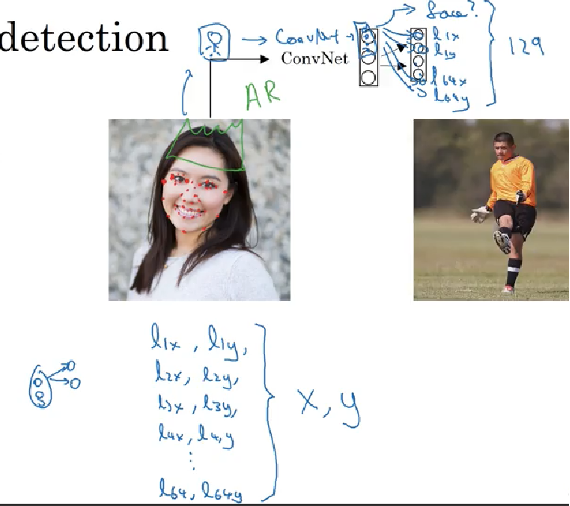
Landmark
- Landmark: you can have neural network just output \(l_X\) and \(l_Y\) of important points and image that you want your neural network model to train.
- 比如recognize eyes, tell all corners of the eyes.
- By Selecting a number of landmarks and generate a label training sets that contains all of these landmarks, you could have neural networks to tell you where are all the key landmarks on a face
- Neural network not only output if it is face or not, also output, \(l_{1X}, l_{1y}; l_{2X}, l_{2y} \cdots\)
- Landmark must be consistent across different images. like One image landmark1 must be left eye left corner, landmark2 must be left eye right corner. Cannot have landmark1 on right eye right corner on different image
- Application: 比如给一个人脸带上皇冠/帽子; specify the pose of the image; recognize emotion
Sliding Windows
- closely cropped image: take a picture, crop out and make car enter d in the entire image or no car in image
- Use ConvNet to recognize if it is car or not for those image
Sliding windows:
- take a small rectangle region, then go through every region of the size(e.g. from top-left to bottom right), pass those little cropped images into ConvNet and make prediction
- Take a slightly larger region and slide the new window with some stride throughout entire image until get to the end, pass those windows into ConvNet and make prediction
- Take a even larger window throughout entire image into ConvNet to make prediction
下图省去了一些中间步骤
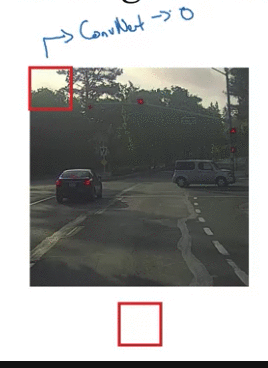
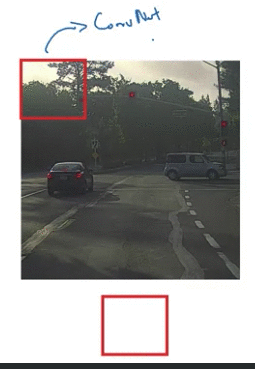
As long as there’s car in the image, there will be a window to detect the car.
Disadvantage: computationtal cost: 因为slide window 太多次to run each of them indepdently through ConvNet,所以花很多时间slide window,
- 但是假如说用一个bigger stride,可能图片没有被captured, hurt performance
- 但如果用小的stride, A huge number of all these regions pass through ConvNet means there is a very high computational cost,also cannot localize objects
- Before, object detection run sliding windows with a simple linear classification is ok. But now, use ConvNet is computational expensive
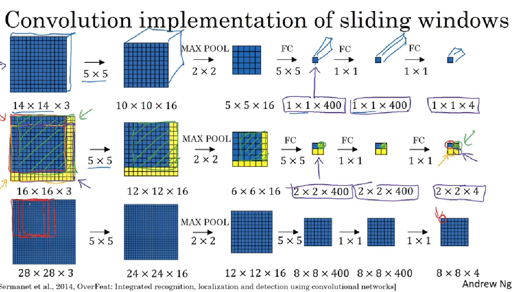
Convolutional Implementation of Sliding windows:
Turning Fully-connected layer into convolutional layers:
5 x 5 x 16fully-connected400 x 1. Now use 400 filters size with ``5 x 5 x 16convolve it to1 x 1 x 400(volume). Mathematically, same as fully connected layer, each number in1 x 1 x 400is some linear function of these5 x 5 x 16` activations from previous layer.- Then implement 1 by 1 convolution with 400 filters size of
1 x 1 x 400 - Then implement 1 by 1 convolutions with 4 filters size of
1 x 1 x 400, and followed by softmax activation and get output size1 x 1 x 4
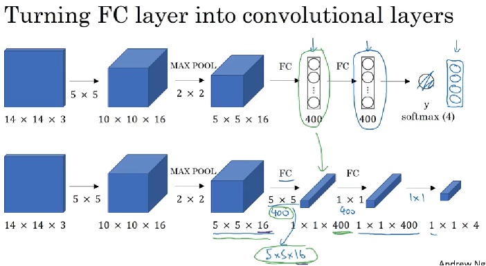
e.g. trainset is 14 x 14 x 3 and test set image is 16 x 16 x 3 image and stride = 2, then slide right two pixel into ConvNet, then move down to ConvNet, finally run right bottom corner window into ConvNet; -> these 4 ConvNets is highly duplicative. So Convolutional implementation of sliding windows is to allow share a lot of computation for those windows
Instead of run four propagation on four subsets of input image independently, it combines all four into one form of computation and shares a lot of the computation in the regions of the image that are common
- the upper-left
2 x 2 x 4gives the result of upper-left corner14 x 14 x 3, the upper-right2 x 2 x 4gives the result of upper-right corner14 x 14 x 3, the upper-left2 x 2 x 4gives the result of lower-left corner14 x 14 x 3, the upper-right2 x 2 x 4gives the result of lower-right corner14 x 14 x 3 - because of max pooling 2 correspond to run your neural network with a stride of two
- weakness: the position of the bounding boxes is not to be accurate
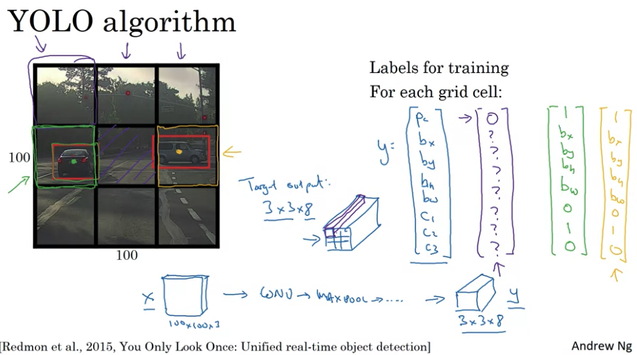
YOLO Algorithm
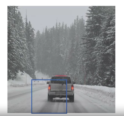
maybe none of boxes really match up perfectly with the position of the car and maybe perfect box is not square, maybe a slightly wider rectangle
YOLO: you only look at once.
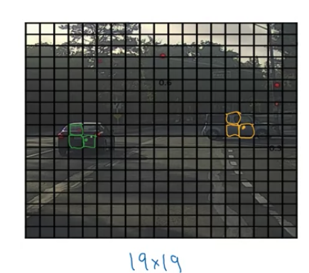
- split image into grid (e.g.
19 x 19grid). If a grid contain object, assigns the object to the grid cell containing the midpoint. 如果一个grid cell 有了车的一小部分,但是假如这个grid cell 没有车的mid point,we assume it does not contain the car- By using
19 x 19grid cell, the chance of an object of two midpoints of objects appearing in the same grid cell is just a bit smaller
- By using
- run through each grid through ConvNet. It’s one single convolutional implementation, not run it grid x grid size times -> efficient algorithm. This works for real time object detection.
- For each grid, output \(y = \begin{bmatrix}P_c \\
b_x \\
b_y \\
b_h \\
b_w \\
b_x \\
c_1 \\
c_2 \\
c_3 \\
\end{bmatrix}\)
- if grid size is
3 x 3, output volume is3 x 3 x 8
- if grid size is
- Advantages: neural network otuput precise bounding boxes for each grid; Convolutional implementation, run fast
- if don’t have more than one object in grid cell, this algorithm works ok
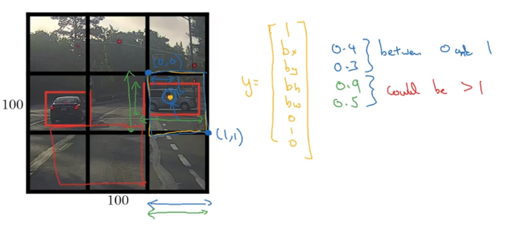
For each grid, use top-left as (0,0) and bottom-right as (1,1), height and width set as fraction of overall height and width of grid cell,(bx, by) (midpoint) has to be less than 1. (bh, b_w) could be larger than 1, because bounding box could be large than grid cell
YOLO Algorithm: put everything together
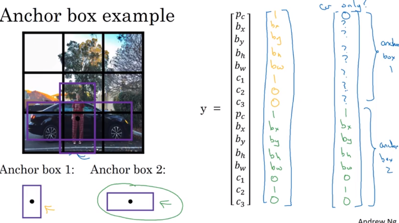
- 对于anchor,真实y 给IoU 最大的anchor box 赋值,其他的anchor box 的pc 赋值为0, 比如下图car more similar to anchor 2 given IoU
- y size is
3 x 3 x 16, for each of nine grid positions, come up with a vector 16 dimensions- In practice, use grid size
19 x 19and 5 anchor boxes, y will be19 x 19 x 40
- In practice, use grid size
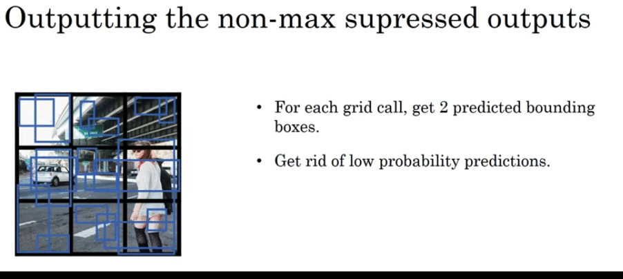
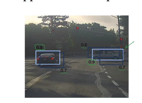
- run with non-max supression to output the non-max supressed output
- if using 2 anchor boxes, for each nine grid box, get 2 anchor boxes. Some of them may have low probability (low \(P_c\)), but still get two bounding box for each nine grid cell
- get rid of low probability prediction
- For each class(predestrian, car, motorcycle) use non-max suppression indepdently to generate final predictions
Note: below picture “For each grid cell” instead of “For each grid call”.
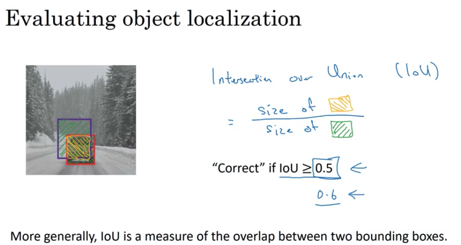
Intersection Over Union
Intersection Over Union(IOU) computes the intersection over union of two bounding boxes(predicted and true labelled).
- Union是 area ideal 的bounding box 和预测的bounding box 全部的面积。Intersection 是 两个图片重合的部分
- IoU= (size of intersection)/(size of union)
- judge output is correct if loU >= 0.5..0,5 is convention. if more stringent, the threshold can be like 0.6/ The higher of the IoU, the more accurate the predicted bounding box. Rare to pick threshold below 0.5
- if the predicted and the ground-truth bounding boxes overlapped perfectly, IoU = 1.
Non-max Suppression
Non-max Suppression: algorithm may find multiple detections of the same object, Non-max Suppression is to make sure you object only be detected only once
some grid may think it can midpoint from the algorithm. End up with multiple detections of each object.
Non-max Suppression: Non-max means you are gonna output the maximal probabilities classification but suppress the close-by ones that are non-maximal
- Discard all boxes with \(P_c \leq 0.6\)
- look at the probability for each detection. Pick the one with the highest \(P_c\)(probability of detection) and highlight this bounding box as prediction
- Look at all remaining bounding box who has a high overlap(high IoU with the one which is highlighted, IoU ≥ 0.5) with the one (highest P_c ) will get suppress/discarded
- Then the highlight one is final prediction
- Repeat the process and select the highest probability which are not suppressed yet
- Carry out non-max suppresion 3 (categories size) times, one on each of pedestrian, car, and motorcycles
Anchor Boxes
之前一个grid 只能预测一个值,但是假如一个grid 有两个我们想预测的值,我们可以用anchor box
e.g. the midpoint of a car and pedestrian fell in the same grid cell
- predefine two different shapes called anchor boxes, then associate two predictions with two anchor boxes
- in practice may use more anchor boxes, e.g. 5 anchor boxes
- use anchor box1 to encode that object and bounding box is pedestrian, use anchor box2 to encode that object and bounding box is car
- With two anchor boxes: each object in training image is assigned to grid cell that contains object’s midpoint and anchor box for the grid cell with highest IoU.
- Anchor boxes compared to ground true bounding box with highest IoU
- object in the training set is labeled as (grid cell, pairs of anchor boxes)
- output y is
3 x 3 x 16, can viewed it as3 x 3 x 2 x 8two anchor boxes
- output y is
- If have more objects, the dimension of Y would be even higher
- Disadvantages:
- Doesn’t handle well if the category of objects in the same grid cell bigger than anchor boxes. (e.g. 3 categories, 2 anchor boxes in a grid cell)
- Doesn’t handle well if two objects have the same anchor box shape in the same grid cell
- It happens quite rarely if two objects appear in the same grid cell, especially
19 x 19grid cell
- Since it is rare two objects in the same grid cell, anchor boxes gives learning algorithm to better specialize. e.g. tall and skinny object like pedestrian, wide and fat object like cars
- How to choose anchor boxes: choose 5 or 10 shapes that spans a variety of shapes to cover the types of objects seem to detect
- Advance version: use K-means algorithm, to group together two types of objects shapes you tend to get, then use that to select a set of anchor boxes that most stereotypciclly representative of multiple objects you’re trying to detect
Previously: each object in training image is assigned to grid cell that contains that object’s midpoint.
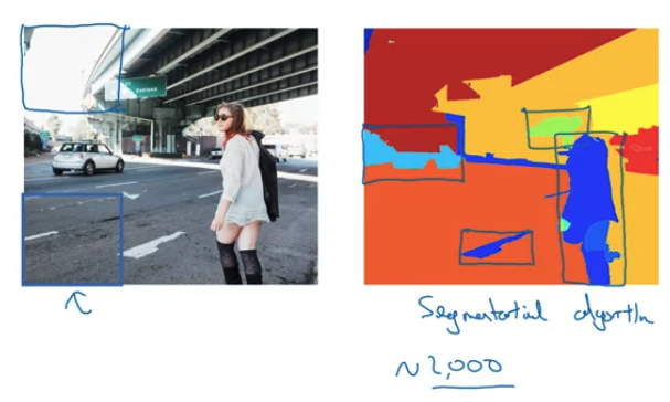
Region Proposal
- When run sliding windows, run detector to see if there’s car, pedestrian or motorcycle. You could run algorithm convolutionaly. Downside of sliding windows: a lot of regions where there’s clearly no object
- Algorithm called R-CNN stands for Regions with convolutional networks or regions with CNNs. It just tried to pick a few regions that make sense to run you convnet classifier rather than running sliding windows on every single window
- Perform the region proposals is to run an algorithm called a segmentation algorithm, pick a bounding box that is more likely to have object. The algorithm may find 2000 blobs/regions and run classifier on those 2000 blobs, which is smaller than run your ConvNet classifier
Faster Algorithms:
- R-CNN:
- propose regions. Classify proposed regions one at a time. Output label + bounding box. RCNN not trust the bounding box which is given, but also output bounding box (\(b_x,b_y,b_h,b_w\))
- Downside: it is quite slow (classify region one at the time)
- Fast R-CNN:
- propose regions. Use convolution implementation of sliding widows to classify all the proposed regions. (use convolutional implementation of sliding windows).
- Downside: the clustering step to propose the regions is still quite slow
- Faster R-CNN: Use convolutional network instead of segmentation algorithms to propose regions. Faster R-CNN implementation are usually still quite a bit slower than the YOLO algorithm
7. Face Recognition
face verification vs. face recognition
- Verification ( 1 to 1 problem)
- input image , name / ID
- output whether the input image is that of claimed person
- Recognition
- has a database of K persons
- Get an input image
- Output ID if the image is any of the K persons ( or “not recognized” )
One Shot Learning
One Shot Learning problem: for most face recognition applications, you need to be able to recognize a person given just one single image. Historically, deep learning don’t work well if have only one training example.
Instead to train softmax to learn 100 people in database, use similarity function
Input: two images, output = d(img1, img2) = degree of difference between images , 如果those two images are the same person, want this output a small number. If two images are different person, want this output a large number
If d(img1, img2) ≤ τ predict they are the “same” person, If d(img1, img2) > τ , predict they are different person. This is to address face verification problem
Use this in recognition, given new pciture, use this function(d(img1, img2)) to compare this new picture and other pictures in the database.
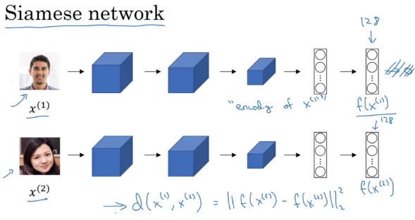
Siamese Network
Pass a image through a sequence of convolutional, pooling, and fully-connected layer and end-up with a feature vector \(f\left( x^{]\left( 1 \right)} \right)\) as encoding of \(x^{]\left( 1 \right)}\) (e.g. size 128 x 1, not pass to softmax unit). Then pass a second image through the same network and get the second encoding \(x^{]\left( 2 \right)}\),
Norm of the difference
\[d\left( x^{\left( 1 \right)}, x^{\left( 2 \right)}\right) = \| f\left( x^{\left( 1 \right)} \right) - f\left( x^{\left( 2 \right)} \right) \|_2^2\]Siamese Neural Network Architecture: run two identical convolutional neural networks on two different inputs and compare them
- these two neural networks have the same parameters
- Parameters of NN define an encoding \(f\left( x^{\left( 1 \right)} \right)\)
- learn parameter that
- if \(x^{\left( i \right)}, x^{\left( j \right)}\) are the same person, \(d\left( x^{\left( 1 \right)}, x^{\left( 2 \right)}\right) = \| f\left( x^{\left( 1 \right)} \right) - f\left( x^{\left( 2 \right)} \right) \|_2^2\) is small
- If \(x^{\left( i \right)}, x^{\left( j \right)}\) are the different person, \(d\left( x^{\left( 1 \right)}, x^{\left( 2 \right)}\right) = \| f\left( x^{\left( 1 \right)} \right) - f\left( x^{\left( 2 \right)} \right) \|_2^2\) is large
- So as you vary the parameters in all of these layers of the neural network end up different encoding, then use back propagation to vary all those parameters in order to make sure these conditions (1,2) are satisfied
Triplet Loss
Learning Objective
Always looking at three images at a time, look at anchor(A) image,positive(P) image(跟anchor 属于一个人的),, negative(N) image(跟anchor 图片不是一个人)
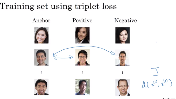
如果f always output zero, will satisfy this equation, to make sure that it doesn’t set all the encodings equal to each other, 所以为了避免这个,我们加上一个α (margin), another hyperparameter, margin does to push anchor positive pair further away from anchor negative pair
\[\| f\left(A \right) - f\left( P \right) \|_2^2 + \alpha \leq \| f\left(A \right) - f\left( N \right) \|_2^2\] \[\| f\left(A \right) - f\left( P \right) \|_2^2 - \| f\left(A \right) - f\left( N \right) \|_2^2 + \alpha \leq 0\] \[\text{Loss Function: } L\left(A,P,N\right) = max\left(\| f\left(A \right) - f\left( P \right) \|_2^2 - \| f\left(A \right) - f\left( N \right) \|_2^2 + \alpha, 0 \right)\] \[\text{Cost Function: } J = \sum_{i=1}^m L\left( A^{\left( i \right)} , P^{\left( i \right)}, N^{\left( i \right)} \right)\]If you have 10k picture with 1000 different persons, then generate/select triplet and then train gradient descent on this type of cost function. you do need multiple pictures for the same person, then you can apply it to one shot learning problem after training (但是training 需要一个人多个图片, if have just one picture of each person, can’t train the system)
Choose the triples A.P.N
During training, if A,P, N are chosen randomly, d(A,P) + α≤d(A,N) is easily satisfied . So choose triplets that’re hard to train on. Choose d(A,P) quite close to d(A,N), so algorithm will try to push d(A,P) down and push d(A,N) up to keep at least a margin of alpha between the d(A,P) and d(A,N)
Commercial face recognition train a fairly large dataset some million images (10 million images)
Andrew Ng 建立: download someone pretrain model from open-source
As Binary Classification Problem
Triplet loss is one good way to learn the parameters of a ConvNet for a face recognition
Another way to train neural network is to take a pair neural networks to take Siamese Network and have them both compute these embeddings \(f\left( x^{\left(i \right) } \right)\) ( maybe 128 feature vector) and use these input to a logistic regression to make prediction, if output = 1, they are the same person whereas output = 0 they are different persons
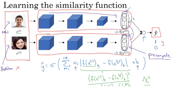
The output \(\hat y\) will be (element-wise difference of encodings)
\[\hat y = \sigma \left(\underbrace{\sum_{k=1}^{128} w_k\mid f\left( x^{\left(i \right) } \right)_k - f\left( x^{\left(j \right) } \right)_k \mid}_{ \text{element-wise difference in absolute values between encodings} } + b \right)\]can think of these 128 numbers as features that you then feed into logistic regression , and train the weight w,b in order to predict whether or not two images are of the same person
There are a few other variations on how to compute \(\hat y\), using \(\chi^2 similarity\)
\[\hat y = \sigma \left( \sum_{k=1}^{128} w_k \frac{ \left( f\left( x^{\left(i \right) } \right)_k - f\left( x^{\left(j \right) } \right)_k \right)^2 } { f\left( x^{\left(i \right) } \right)_k + f\left( x^{\left(j \right) } \right)_k } + b \right)\]One single trick is to precompute the feature vector(通过Siamese network算出来)in the database to save computational cost (not need to store raw image). This works for Siamese Network where treat face recognition as a binary classification problem or when you were learning encodings using Triplet Loss function
8. Neural Style Transfer
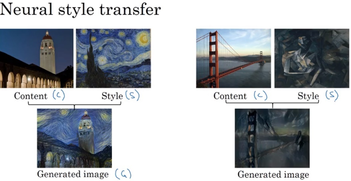
Neural Style Transfer: generate image from content image but drawn in the style of the style image
What are deep ConvNets learning?
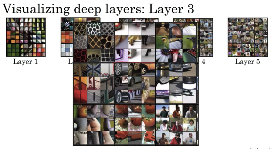
e.g. Pick a unit in layer 1. Find the nine different image patches(3 x 3 ) that maximize the unit’s activation (there are many activations in layer1). pass training set into neural network and figure out what is the image that maximizes that particular units activation. By doing this, will see what is hidden layer recognizing such as looking for simple features like a veritical line
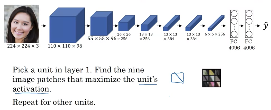
In the deeper layer, a hidden unit will see a larger region of the image. Each pixel could hypothetically affect the output of later layers of neural network. Later units are actually seen larger image patches.
Cost Function
\[J\left(G \right) = \alpha J_{content}\left(C,G \right)+\beta J_{style} \left(S,G \right)\] \[\text{G:generated image; C: content image; S: style image}\]\(J_{content}\left(C,G \right)\) measures how similar content image to generated image, \(J_{style} \left(S,G \right)\) measures how similar style image to generated image. \(\alpha, \beta\) two hyperparameters to specify relative weighting for content cost and style cost.
Find the generated image G:
- Initiate G randomly. might be G:
100 x 100 x 3. Initialize G just white noise image with each pixel value chosen at random - Use gradient descent to minimize J(G) , \(G := G - \frac{\partial}{\partial G} J\left( G \right)\) to slowly update the pixel value so get an image that looks more and more like content image rendered in style image
- In the process, actually updating the pixel values of image G
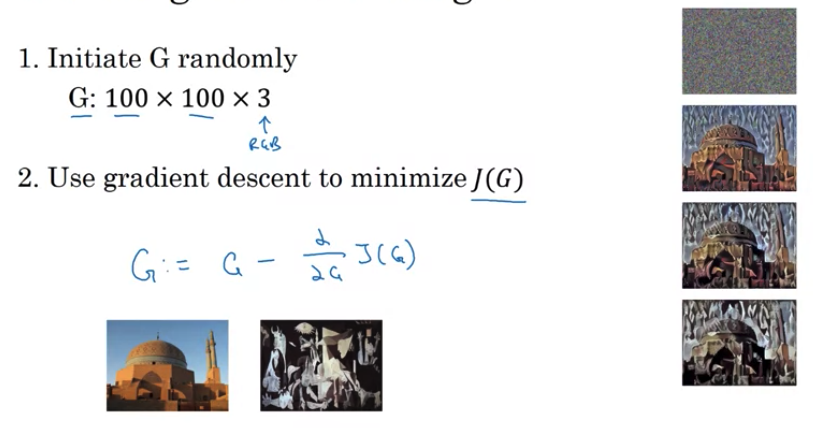
Overall Cost Function: use gradient descent or sophisticated optimization algorithm in order to try ot find an image G that minimize the cost function \(J\left( G \right)\)
\[J\left(G\right) = \alpha J_{content} \left( C,G\right) + \beta J_{style} \left( S,G\right)\]Content Cost Function
- Say you use hidden layer l to compute content cost
- if l is a small number, hidden layer 1, it will force your generated image pixel values very similar to content image.
- if l is a large number, a deep layer. If there is a dog in your content image, it will generate dog somewhere in the generated image
- In practice, l is chosen neither too shallow nor too deep in the neural network. l is chosen in the middle layer of the neural network
- Use pre-trained ConvNet (E.g, VGG network)
- Let \(a^{\left[ l \right]\left( C \right)}\) and \(a^{\left[ l \right]\left( G \right)}\) be the activation of layer l on the images
- if \(a^{\left[ l \right]\left( C \right)}\) and \(a^{\left[ l \right]\left( G \right)}\) similar, imply both images have similar content
- 有没有1/2都可以, element wise sum of square difference between activations of C and G
Style Cost Function
Say you are using layer l’s activation to measure “style”. Define style as correlation between activations across channels
the correlation tells you which of these high level texture components tend to occur or not occur together in part of an image. And degree of correlation gives measuring how often in generated image these different high level features come together or not such as 第一个 channel activation 识别 vertical texture 与 第二个channel activation 识别 orange tint correlate
Style Matrix
Let \(a_{i,j,k}^{\left[ l \right]} =\) activation at (i,j,k), i is height, j is width, and k is channel. \(G^{\left[ l \right]}\) is \(n_c^{\left[ l \right]} \times n_c^{\left[ l \right]}\) dimension matrix (Squared matrix). You can \(n_c\) channel so \(G^{\left[ l \right]}\) measure how correlated each pair of them is. \(G_{k, k'}^{\left[ l \right]}\) meaures how correlated activations in channel k compared to the activations in channel k’. k is range \(\left[1, n_c \right]\)
For style image
\[G_{k, k'}^{\left[ l \right] \left( S \right) } = \sum_{i=1}^{n_H^{ \left[ l \right] }}\sum_{j=1}^{n_W^{ \left[ l \right] }}a_{i,j,k}^{\left[ l \right] \left( S \right)} a_{i,j,k'}^{\left[ l \right] \left( S \right)}\]For generated image
\[G_{k, k'}^{\left[ l \right] \left( G \right) } = \sum_{i=1}^{n_H^{ \left[ l \right] }}\sum_{j=1}^{n_W^{ \left[ l \right] }}a_{i,j,k}^{\left[ l \right] \left( G \right)} a_{i,j,k'}^{\left[ l \right] \left( G \right)}\]In linear algebra, style matrix also called gram matrix
If \(a_{i,j,k}^{\left[ l \right]} a_{i,j,k'}^{\left[ l \right]}\) correlate, \(G_{k, k'}^{\left[ l \right]}\) will be larger. If \(a_{i,j,k}^{\left[ l \right]} a_{i,j,k'}^{\left[ l \right]}\) uncorrelate, \(G_{k, k'}^{\left[ l \right]}\) will be small.
\[J_{style}^{\left[ l \right]} \left( S,G \right) = \frac{1}{ \left( 2 n_H^{ \left[ l \right] } n_w^{ \left[ l \right] } n_c^{ \left[ l \right] } \right)^2} \| G^{\left[ l \right] \left( S \right)} - G^{\left[ l \right] \left( G \right)} \|_F^2 \text{ Frobenius norm}\] \[J_{style}^{\left[ l \right]} \left( S,G \right) = \frac{1}{ \left( 2 n_H^{ \left[ l \right] } n_w^{ \left[ l \right] } n_c^{ \left[ l \right] } \right)^2} \sum_{k=1}^{n_c }\sum_{k'=1}^{ n_c } \left( G_{k, k'}^{\left[ l \right] \left( S \right) } - G_{k, k'}^{\left[ l \right] \left( G \right) } \right)^2 \text{ Frobenius norm}\]This is just the sum of squares of element wise differences between two matrices
Overall Style Cost Function
\[J_{style} \left( S,G \right) = \sum_{l} \lambda^{\left[ l \right]}J_{style}^{\left[ l \right]} \left( S,G \right)\]\(\lambda\) are a set of hyperparameters. It allows you to use different layers in neural network, in lower layer simple low level features (early one) whereas in latter layer measure high level features and cause neural network to take both low level and high level features to take into account when computing style
1D and 3D Generalizations
1D
1D time series data. Take the 1D filter and similarly apply that in lots of different positions throughout 1D data
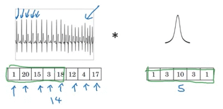
e.g.
\[\require{AMScd} \begin{CD} \text{14 dimension 1D} @>{\text{1 D 16 filters size of 5}}>> 10 \times {16} \text{dimension} \end{CD}\]3D
Instead of having 1D listor 2D matrix of numbers, now have 3 D block, a three dimensional input volume of numbers
3D 要考虑 height, width and depth(height, width, and depth can be dfiffeent), filter also need to be 3 D (height, width, depth)
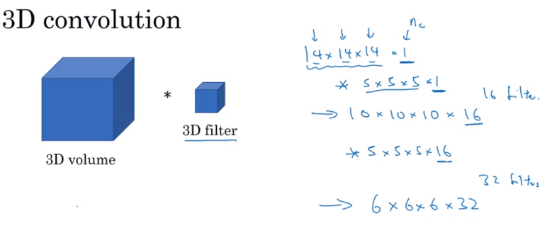
what filters do is rally to detect across your 3D data
e.g. Movie data where the different slices could be different slices in time through a movie. could use this to detect motion or people taking actions in movies
9 Paper for Reference
- Gradient-Based Learning Applied to Document Recognition, Yann LeCun, 1998: LeNet5
- ImageNet Classification with Deep Convolutional Neural Networks , Alex Krizhevsky, 2012: AlexNet
- Very Deep Convolutional Networks for Large-Scale Image Recognition , Karen Simonyan, Andrew Zisserman, 2016: VGG - 16
- Deep Residual Learning for Image Recognition, Kaiming He, Xiangyu Zhang, Shaoqing Ren, Jian Sun, 2015: ResNet
- Network In Network, Min Lin, Qiang Chen, Shuicheng Yan, 2013: 1 x 1 Convolutions
- Going Deeper with Convolutions, 2014 Inception Network
- You Only Look Once: Unified, Real-Time Object Detection, Redmon 2015: YOLO Algorithm
- Rich feature hierarchies for accurate object detection and semantic segmentation, Girshik, 2014: Regional Proposals
- DeepFace: Closing the Gap to Human-Level Performance in Face Verification, Taigman, 2014
- FaceNet: A Unified Embedding for Face Recognition and Clustering, Schroff, 2015: Face Recognition, Triplets loss
- Visualizing and Understanding Convolutional Networks Matthew D Zeiler, Rob Fergus: What are deep ConvNets Learning
- A Neural Algorithm of Artistic Style: Neural Style Transfer Cost Function