Machine Learning

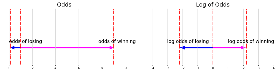
Logit Function

\[Odd = \frac{P }{1- P}, \text{ where p is probability}\] \[\color{fuchsia}{\bf{odd} = \frac{\text{Something happening i.e. wining}}{ \text{Something not happening. i.e. losing }}}\] \[\color{blue}{\bf{probability} = \frac{\text{Something happening i.e. wining}}{ \text{everything could happen. i.e. losing + winning}}}\]

P is the probability and odds is not probability. E.g. Winning a game probability is 0.7, Odds of winning is: $Odd = \frac{7}{3}$

Log of odds: the asymmetry of odds make it diffcult to compare the odds for something happening or not happening.

\[- log \left( \frac{p}{1-p} \right) = log \left( \frac{1-p}{p} \right)\]

E.g. If the probability of winning is 0.9, the odds of winning is 9, the odds of losing $\frac{1}{9}$

Derived Sigmoid Function

\[\begin{aligned} log \left( \frac{p}{1-p} \right) &= W X + b \\ \frac{p}{1-p} &= e^{WX + b} \\ p &= e^{WX + b} - p e^{WX + b} \\ P &= \frac{e^{WX + b}}{ 1 + e^{WX + b}} \\ &= \frac{1}{ 1 + e^{-\left(WX + b\right)}} \\ \end{aligned}\]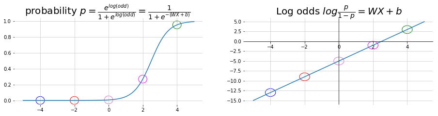

Decision Tree

Advantage: easy to use / train and easy to interpret.
Disdvantage: not flexible when comes to classifying new samples, often being overfit

Entropy: a measure of disorder or uncertainty. High Value means high disorder.

\[E\left(S \right) = -\sum_{i=1}^c P\left( x_i \right) log_2 P\left( x_i \right)\]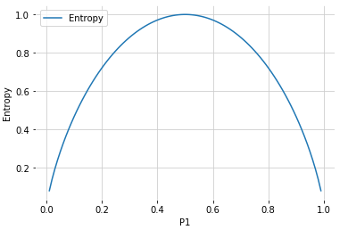

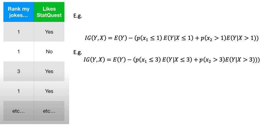
Information Gain: the higher the value, the more gains

Decision Trees algorithm will always tries to maximize Information gain.
An attribute with highest Information gain will tested/split first.

\[\begin{aligned} IG \left(Y,X \right) &= E\left( Y \right) - E \left( Y \mid X \right) \\ & = E \left( Y \right) -\big( p\left( x_1 \right) E \left( Y \mid X = x_1 \right) + p\left( x_2 \right)E\left( Y \mid X= x_2 \right) \big) \end{aligned}\]

e.g. Use if height is bigger than 190 cm to predict if a person is a NBA player

Height > 190cm (X)	Is NBA player (Y)
Yes	Yes
No	Yes
Yes	No
No	No
Yes	Yes

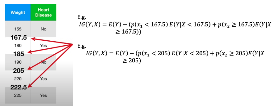
\[E(Y) = - \frac{2}{5} * log_2 \left( \frac{2}{5} \right) - \frac{3}{5} * log_2 \left( \frac{3}{5} \right) = 0.971\] \[E(Y | X = Yes) = - \frac{1}{3} * log_2 \left( \frac{1}{3} \right) - \frac{2}{3} * log_2 \left( \frac{2}{3} \right) = 0.918\] \[E(Y | X = NO) = - \frac{1}{2} * log_2 \left( \frac{1}{2} \right) - \frac{1}{2} * log_2 \left( \frac{1}{2} \right) = 1\] \[\begin{aligned} IG \left(Y,X \right) &= E\left( Y \right) - \big( p\left( X=YES \right) E \left( Y \mid X = YES \right) + p\left( X = No \right)E\left( Y \mid X= NO \right) \big) \\ &= 0.971 - \left( \frac{3}{5} *0.918 + \frac{2}{5}*1 \right) \\ &= 0.02 \end{aligned}\]

For Numerical Values, Sort the value, calculate the average for all adjacent points, then use each average value as the threshold to compute information gain and find the best one

When dealing with rank values. Try each rank as threshold and find the best one. e.g. only has 1 to 4 rank. Note: 不用试 rank = 4 as threshold 因为所有rank 都小于4

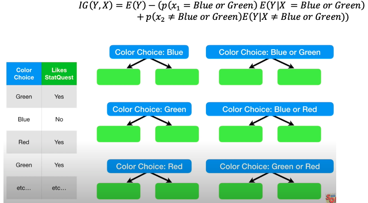
When dealing with multiple categorical values: Try each possible combination and find the best one

Regression Tree

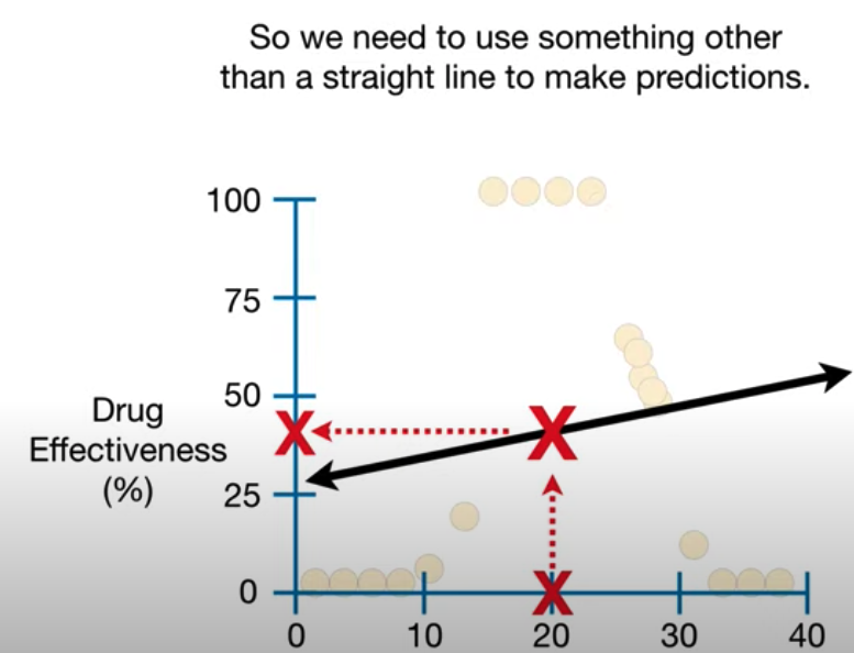
The failure of Linear Regression:

Regression Tree are a type of decision tree.
- In regression tree, each leaf represents a numeric value
- Classification Trees have True or False or some discrete category in their leaves
Regression Tree easily accomodates additional predictors
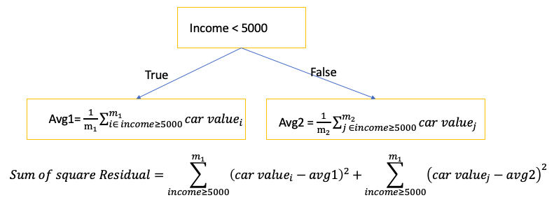
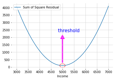
To find the threshold for each node: split the data into two groups by finding the threshold that gave the smallest sum of squared residuals $\sum \left( predicted - observed \right)^2$
When there are multiple features, try different features with different threshold. Then use the feature with the threshold that has the smallest sum of squared residuals as the node and threshold
The leaf values is the average of observation values ending within this leaf
If each leaf end with only one observation, the accuracy of training is 100% but it will overfit the training data. To aviod overfitting:
1. Only split observations when there are more than some minimum number. Typically the minimum number of observations to allow for a split is 20
2. Remove some of leaves and combine them into one leaf. The predicted value of the leaf is the average of all values

E.g. Use employee’s Income to predict car value

Cost Complexity Prune Tree

How to prune the tree to avoid the overfitting on training data (not perform so well on training data )
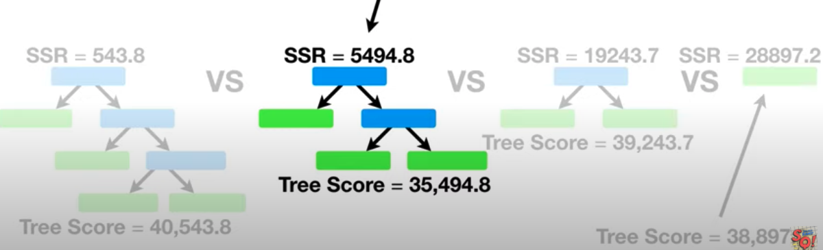
Tree Score: based on Sum of Squared Residuals (SSR) for the tree or sub-tree and Tree Complexity Penalty(T) that is a function of the number of leaves, or Terminal nodes in the tree or sub-tree
- Tree Complexity Penalty compensates for the difference in the number of leaves
- $\alpha$ is a tuning parameter. Find the best $\alpha$ using cross validation

\[\bf{\text{Tree Score } = SSR + \alpha \underbrace{T}_{\# Leaves}}\]

e.g. tree has four leaves and $\alpha = 10000$

\[\bf{\text{Tree Score }} = 543.8 + 10000 \times 4\]

Step 1: Tunning $\alpha $ using use all of the data (not just training)

build the full-sized regression Tree (which do the best on training data). It has the lowest Sum of Squared Residuals among all the trees($\alpha = 0$)
Increase $\color{red}{\bf{\alpha}}$ until pruning leaves(reducing number of leaves) give us a ower Tree score
Repeat Step 2. then different values for $\color{red}{\bf{\alpha}}$ give a sequence of trees from full sized to just a leaf. (每个tree 对应一个 $\alpha$)

Step 2: Selecting the best $\alpha$. Divide data into training and testing.

Use the $\alpha$ found at the step 1 to build a full tree and a sequence of subtrees that minimize the Tree Score for each sub-tree
Repeat above step K times (K-fold cross validation), then pick the $\alpha$ which has lowest average Sum of Square Residuals with Testing Data (如果有N 个tree, 有N个$\alpha$对应，选择最小的average Sum of Square Residuals的 $\alpha$)

Step 3: pick the tree build at Step 1(with full data) that corresponds to the value for $\alpha$ selected at Step 2 as the final pruned tree

Random Forest

Random Forest combine the simplicity of decision tress with flexibility resulting in a vast improvement in accuracy.

Build Random Forest

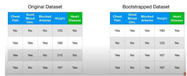
Step 1: Bootstrap Create new dataset, same size as original, randomly select samples from original dataset and allows duplicate

Bagging:combine classifiers by sampling/bootstrapping training set
Out-of-bag dataset: Around 1/3 of original data doesnot end up in the bootstrap dataset

Step 2: Create a decision tree using the bootstrapped dataset but only use a random subset of variables at each step

e.g. total features = 4 at first node, only randomly select 2 out of 4 features to see which one of 2 is best for the first node. Then to select second nodes, randomly select 2 out of 3 features to see wich is the best

Step 3: Repeat step 1 and 2 N times, and generate a wide variety of trees.

The variety makes random forests more effective than individual decision trees.

Evaluation

run all out-of-bag samples for all of trees and see if the predictions are correct or not.

For each evaluation sample, run through all N trees and use the most predicted class as output
- e.g. total 100 trees, 80 of them predict a person is a NBA player and 20 of them predict not NBA player. Output = NBA player

\[Accuracy = \frac{\text{correct labeled prediction for out-of-bag dataset}}{\text{total out-of-bag size}}\] \[\bf{\text{Error of out-of-bag samples}} = \frac{\bf{\text{incorrect}} \text{ classification for out-of-bag dataset}}{\text{total out-of-bag size}}\]

e.g. total 100 out-of-bag size, 80 of them predict correct(running all trees, label is same as most predict classes), Accuracy = 0.8

Missing Values

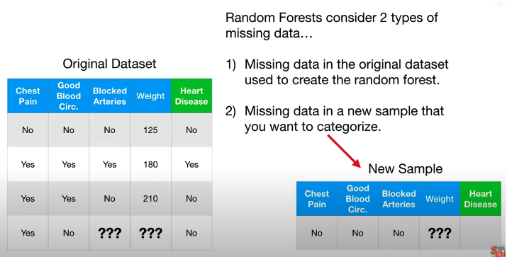
Deal with missing data in original dataset

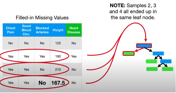
Step 1: Make a initial guess:

For categorical value: guess the common class among other samples that have the same label.
For numeric value: guess the median value among other samples that have the same label.
- e.g. In above picture, label of missing row No Heart Disease, then find for other No Heart Disease sample, the median of weight is (125 + 210)/2 = 167.5

Step 2: Build the random forest using all samples including guessed ones:

Step 3: Run all of data for all the tree and build Proximity Matrix

\[\text{Proximity value} = \frac{\color{fuchsia}{\text{the number of times two data end with the same leaf node}}}{\text{total random forest trees}}\] \[Distance = 1- \text{Proximity value}\]

If Distance close to 0, means two data end with teh same leaf node for all trees

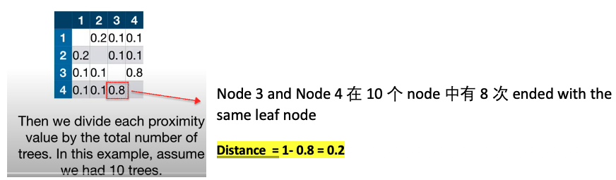
Step 4: use the proximity values to make better guess about the missing data

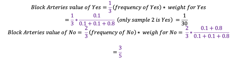
Because $\frac{3}{5} > \frac{1}{30}$, esitmated value is no

\[\begin{aligned} \text{Weight Guess} &= 125*\frac{0.1}{0.1+0.1+0.8} \\ & +180*\frac{0.1}{0.1+0.1+0.8} \\ & + 210*\frac{0.8}{0.1+0.1+0.8} = 198.5 \end{aligned}\]

Step 5: Repeat step 1 and 3 over and over again to build the tree, run the data through the tree, and recalculate the missing value until missing value converge. No longer change each time we recalculate

Deal with missing data in new sample that need to be predicted

Step 1: Create n (total n classes) copies of the data, one for each predicted class`

e.g. data is missing for height > 190cm. Make 2 copies of data, and label the first is NBA player and another second not a NBA player

Step 2: use above iterative methods to make a good prediction about the missing values for each copy of labeled class

e.g. guess height > 190cm for both copies

Step 3: Then run those n copies of data through the trees in the forest with filled estimation value, and see which one is correctly labeled by the random forest the most times

e.g. total 100 trees, Predict 80 as NBA player for the one labeled as NBA player. Predict 60 as not NBA player for the one labeled as not a NBA player. Finally output as NBA player

AdaBoost

Random Forest, make a full size tree and some tree may bigger than others
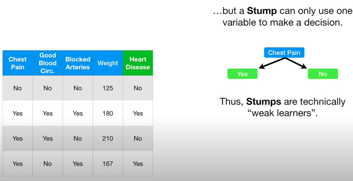
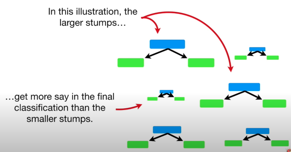
In a Forest of Trees made with AdaBoost, the trees are usually just a node and two leaves(called Stump)
- Stump are not great at making accurate classifications
AdaBoost combines a lot of weak learners(stumps) to make clasfication
Some Stumps get more say in the classification than others
Each stump is made by taking previous stump’s mistakes into account
In practice, we usually stop boosting after certain iterations to both save time and prevent overfitting

In Random Forest, each tree has an equal vote on the final classification. However for AdaBoost in a Forest of Stumps, some stumps get more say in final classification than others

In Random Forests, each decision tree is made independently of the others. In contrast, in a Forest of Stumps made with AdaBoost, order is important

The error of first stump made influence how second stump made. Then error of second stump influence the third stump.

Create a Forest of Stumps using AdaBoost

Step 1: Give each sample a weight that indicates how important it is to be correctly classified. At start, all sample get a same weight.

\[weight = \frac{1}{\text{total number of samples }}\]

Step 2: Then choose the best feature as the node of stump

Step 3: Calculate Total Error and Amount Say for the stump. Total Error is always between 0 and 1. 0 is perfect stump and 1 for horrible stump

when stump does a good job, Total Error is small and Amount of Say is large
When stump like flipping a coin, Total Error = 0.5 and Amount of Say is 0
When stump consistently gives the opposite classification, Total Error is close to 1 and Amount of Say is a large negative value

\[\text{Total Error} = \frac{\text{total data being incorrectly classified}}{\text{total number of dataset}}\] \[\text{Amount of Say } \left( \alpha_t \right) = \frac{1}{2} log\left( \frac{1 - \text{Total Error}}{\text{Total Error }} \right)\]

Step 4: Use the amount of say to Adjust the weight. The idea is to increase weight for incorrectly classified sample and decrease weight for correctly classified sample

\[\text{Incorrectly classified Sample Weight} = \text{sample weight} \times \color{fuchsia}{e^{\text{amount of say}}}\] \[\text{correctly classified Sample Weight} = \text{sample weight} \times \color{fuchsia}{e^{-\text{amount of say}}}\]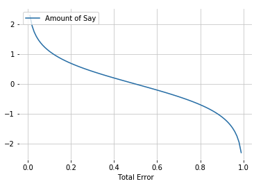

For incorrectly classfied sample:
- If amount of say is large (stump does a good job), new Sample weight will be much larger than old one
- If amount of say is small (stump does not do a good job), new Sample weight will be a little larger than old one
For correctly classfied sample:
- If amount of say is large, new sample weight will very small
- If amount of say is small, new sample weight will very a little smaller than the old one

Step 5: Normalize new weights to make them add to 1

Combine step 4 and step 5:

\[\begin{aligned} W_{t+1}\left( i \right) & = \frac{W_{t}\left( i \right)}{Z_t} \times \begin{cases} e^{-\alpha_t} & \text{if } h_t\left( x_i \right) = y_i \\ e^{\alpha_t} & \text{if } h_t\left( x_i \right) \neq y_i \end{cases} \\ & = \frac{W_{t}\left( i \right) exp\left( -\alpha_t y_i h_t\left(x_i\right) \right) }{Z_t} \\ \text{where } Z_t & = \sum_i W_{t+1}\left(i\right) \\ y_i h_t\left(x_i\right) & = 1 \text{ only if prediction is correct} \\ \end{aligned}\]

where $h_t\left( x_i \right)$ is the prediction of stump, both $h_t\left( x_i \right)$ and $y_i$ only take 1 or -1

Step 6: Gnerate sample based on the new noralized weight(allow duplicate and the same size as before): incorrect classified data will be drawn with a higher probability since the weight is higher

Step 7: Use new genereated sample as dataset and change the weight to equal weight

Note: equal weight doesn’t mean stump will not emphasize the need to correctly classify these samples. Because allow duplicate, in new generated sample there is more data of being incorrectly classfied before

\[weight = \frac{1}{\text{total number of samples }}\]

Or Substitution of Step 6 and 7: use new weight in Information gain/Weighted Gini Function mismatches without generating new dataset

Step 8: Repeat step 1-7 N times to make N stumps

So error of first tree influence second tree, then second tree error influence third tree

Evaluation:

Use the data to pass all the stump and calculate the total amount of say(created during the training) from each predicted class, the class with total largest of amount of say is the prediction class

\[\hat y = sign \left( \sum_{t=1}^T \alpha_t h_t \left(x \right) \right), \text{ T is the number of total Stump}\]

Example

Bagging Vs Boosting

Both have final prediction as a linear combination of classifiers
Bagging combination weights are uniform; boosting weights (amount of say $\alpha_t$) are a measure of performance for classifier at round
Bagging has independent classifiers, boosting ones are dependent of each other
Bagging randomly selects training sets; boosting focuses on most difficult points

Gradient Boost

Pros:

Often best-off-shelf accuracy on many problems
Using modle for prediction requires only modest memory and is fast
Doesn’t requre careful normalization of features to perform well
Like decision trees, handles a mixture of feature types

Cons:

Like Random Forest, the model are difficult for humans to interpret
Requires careful tuning of the learning rate and other parameters
Training can require significant computation
Like Decision trees, not recommended for text classification and other problems with very high dimensional sparse features, for accuracy and computational cost reasons

Gradient Boost for Regression

Gradient Boost starts by making a single leaf, instead of a tree or stump. The leaf represents an initial guess for the Weights of all of the samples
Like Adaboost, Gradient Boost builds fixed sized trees based on the previous tree’s errors
Like Adaboost, Graident Boost scale the trees, However, Gradient Boost all the trees by the same amount
- Gradient Boost use a Learning Rate(Value between 0 and 1) to scale the contribution from the tree instead of Amount of Say
Gradient Boost usually uses trees larger than stumps, In practice, people often set the maximum number of leaves to between 8 and 32
Gradient Boost continues to build trees until it has made the number of trees you asked for or additional trees fail to improve the fit

Algorithm

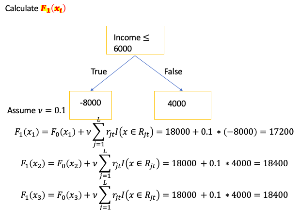
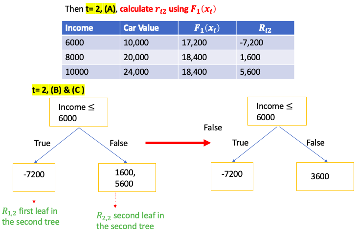
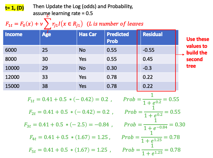
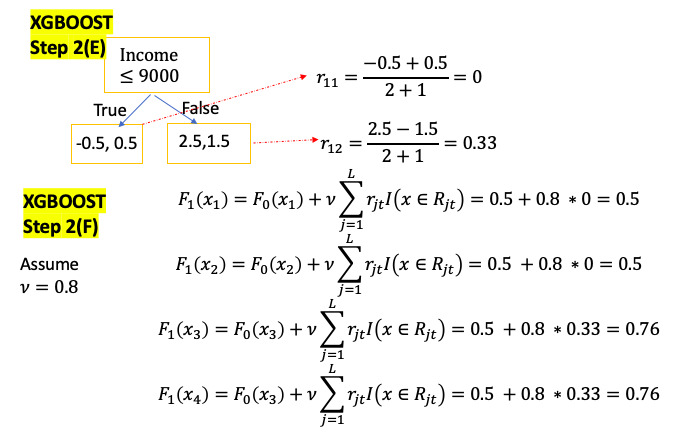
\[\begin{aligned} Input: & Data \{ \left( x_i , y_i \right) \}_{i=1}^m, \text{and a differentiable Loss Function} L \left( y, F\left( x \right) \right) \\ \text{Step 1: } & \text{Initialize model with a constant value } \color{Fuchsia}{F_0\left(x \right) = argmin_\gamma \sum_{i=1}^n L \left( y_i, \gamma \right)}\\ \text{Step 2: } & \text{ for } t = \text{1 to T}: \color{Gray}{\text{( T is the number of Trees)}} \\ & \left( A \right) \text{Compute } \text{ for i = 1...M} \color{Gray}{\text{( M is the number of data)}} \\ & \quad \color{Fuchsia}{r_{it} = - \left[ \frac{\partial L \left( y_i, F\left( x_i \right) \right)}{\partial F\left( x_i \right)} \right]_{F\left( x \right) = F_{t-1}\left( x \right)}} \\ & \left( B \right) \text{Fit a regression tree to pseudo-residuals, train it using } \left( x_i , r_{it} \right) \}_{i=1}^m \\ & \quad \text{and create Terminal regions } R_{jt} \color{grey}{\text{( j-th leaf in the t-th tree)}} \\ & \left( C \right) \text{For j = 1 ... L compute } \color{Fuchsia}{r_{jt} = argmin_\gamma \sum_{x_i \in R_{jt}} L \left( y_i, F_{t-1}\left( x_i \right) + \gamma \right)} \\ & \quad \color{grey}{\text{( L is total number of leaves in t-th tree )}} \\ & \left( D \right) \text{update the model }, \nu \text{ is learning rate} \color{grey}{\text{ (value between 0 and 1)}}\\ & \quad \color{Turquoise}{F_t\left( x \right) = F_{t-1}\left( x \right) + \nu \sum_{j}^L r_{jt} I\left( x \in R_{jt} \right)} \\ \end{aligned}\]

Explanation:: $\hat y_i = F_i \left( x \right)$ : ith tree prediction value

Input: Data $\{ \left( x_i , y_i \right) \}_{i=1}^m$, and a differentiable Loss Function $L \left( y_i, F\left( x \right) \right)$

$\{ \left( x_i , y_i \right) \}_{i=1}^m$ m is the number of training data, and $x_i$ is a vector represent input features. $y_i$ is the predicted value
Loss Function $L \left( y, F\left( x \right) \right) = \frac{1}{2} \sum_{i=1}^m \left( y_i - F\left( x \right)\right)^2$, m is total number of data

Step 1

\[F_0\left(x \right) = argmin_\gamma \sum_{i=1}^m L \left( y_i, \gamma \right)\]

means need to find a $\gamma$ value to minimize the sum of Loss function. Can calculate the derivative of Loss function respect to $F_0\left(x \right)$. And set it equal to 0 to find the optimal value

It is average of y. It means the prediction just the averge of y of training data.
Only $F_0\left(x\right) $ is the same for all $x_i$. Once update the $F_t\left(x_i \right) $ using pseudo-residual, $F_t\left(x_i \right) $ will be different for differernt $x_i$

\[\frac{d }{d F_0\left(x \right)}\sum_{i=1}^m L \left( y_i,F_0\left(x \right) \right) = \frac{d }{d F_0\left(x \right)}\sum_{i=1}^m \frac{1}{2} \left( y_i - F_0\left(x \right) \right)^2 = - \sum_{i=1}^m \left( y_i - F_0\left(x \right) \right)\] \[- \sum_{i=1}^m \left( y_i - F_0\left(x \right) \right) = 0 \Rightarrow F_0\left(x \right)= \frac{1}{m}\sum_{i=1}^m y_i\] \[F_0\left(x \right) = \frac{1}{m}\sum_{i=1}^m y_i\]

T is the number of Trees and usually set to 100 trees

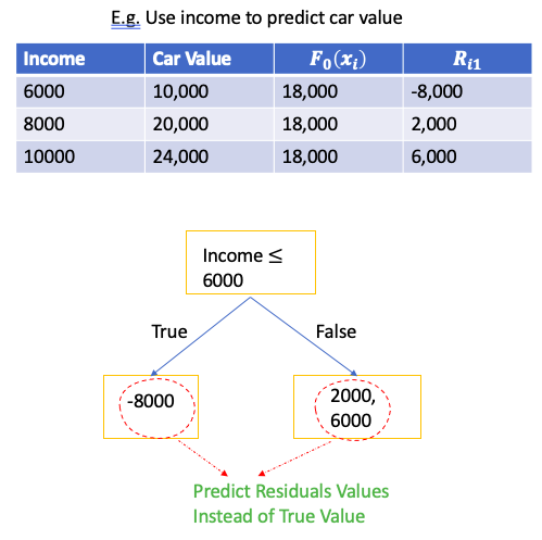
(A): $r_{it}$: t-th tree’s i-th sample Pseudo Residuals

for i = 1, … , m is to calculate residual for all the samples in the dataset

\[r_{it} = - \underbrace{ \left[ \frac{\partial L \left( y_i, F\left( x_i \right) \right)}{\partial F\left( x_i \right)} \right]_{F\left( x \right) = F_{t-1}\left( x \right)}}_{\text{Plug last step } F\left(x \right) \text{ into equation after getting the derivative}}\]

As we know,

\[- \frac{\partial L \left( y_i, F\left( x_i \right) \right)}{\partial F\left( x_i \right)} = - \frac{d }{d \hat y} L \left( y_i, F\left(x_i \right)\right) = y_i - F\left(x_i \right)\]

When t = 1,

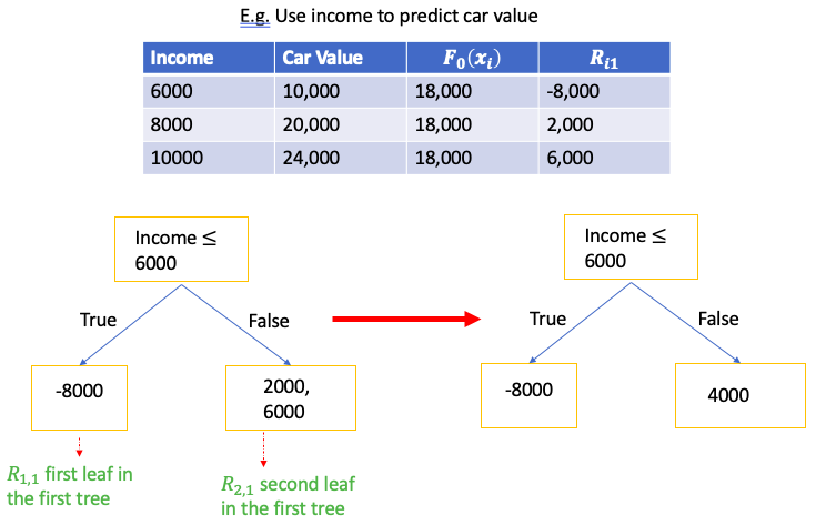
\[y_i - F_0\left(x_i \right) = y_i - \text{average of y}\]

(B): means to build a regression tree to predict residuals instead of true y value

(C): if multiple training data end with the same leaf, use this equation to calculate output value. Calulate the derivate of Loss function respect to $F_{t-1}$, and set it to 0 to find the optimal value

Each time add a tree to the Prediction, the residuals get smaller

\[\sum_{x_i \in R_{jt}} L \left( y_i, F_{t-1}\left( x_i \right) + \gamma \right) = \sum_{x_i \in R_{jt}} \frac{1}{2} \left( y_i - \left( F_{m-1}\left( x_i \right) + \gamma\right) \right)^2\] \[\frac{d}{d \gamma} \sum_{x_i \in R_{jt}} \frac{1}{2} \left( y_i - \left( F_{m-1}\left( x_i \right) + \gamma\right) \right)^2 =\] \[\begin{aligned} \frac{d}{d \gamma} \sum_{x_i \in R_{jt}} \frac{1}{2} \left( y_i - \left( F_{m-1}\left( x_i \right) + \gamma\right) \right)^2 & = -\sum_{x_i \in R_{jt}} \left( y_i - F_{m-1}\left( x_i \right) - \gamma \right) \\ &= -\sum_{x_i \in R_{jt}} \left( \text{pseudo residual} - \gamma\right) \end{aligned}\] \[\gamma = \frac{1}{\text{number of sample end in } R_{jt}} \sum_{x_i \in R_{jt}} \text{pseudo residual}\]

(D): make a new prediction for each sample. Each new prediction is based on last prediction made and the tree just making

A small learning rate reduces effect each tree has on the final prediction and this improves accuracy in the long run

Gradient Boost for Classification

Same algorithm as Regression but cost function changes. Some detailed explanation below.

$F_0 \left( x \right)$ is the log odds
Each leaves output is log odd . Whereas, in Gradient Boost for Regression, a leaf is the average of Residual

Convert Log(odds) to probability

\[P = \frac{e^{log\left(odd\right)}}{1+ e^{log\left(odd\right)}} = \frac{1}{1+ e^{-log\left(odd\right)}}\]

Convert probability to Log(odds)

\[Log\left( odds \right) = \frac{\sum_{\color{red}{leaf}} Residual_i}{\sum_{\color{red}{\text{leaf}}} \text{Previous Probability } \times \left( 1-\text{Previous Probability } \right) }\]

Evaluation:

\[Log\left( odds \right) = F_0 \left( x_i \right) + \nu F_1 \left( x_i \right) + \cdots + \nu F_T \left( x_i \right)\]

Then Predict

\[y = \begin{cases} 1 & \text{ if } \frac{1}{1 + e^{-Log\left( odds \right)}} > 0.5 \\ 0 & \text{ if } \frac{1}{1 + e^{-Log\left( odds \right)}} \leq 0.5 \\ \end{cases}\]

Input: Data ${ \left( x_i , y_i \right) }_{i=1}^m$, and a differentiable Loss Function $L \left( y_i, F\left( x \right) \right)$

$y_i$ is the categorical value
Loss Function of Binary classification : $ F\left( x \right)$ refers as predicted probability.
The goal is to maximize the loglikehood function and minimize loss function. So if want to use loglikehood function as cost function, multiply by -1

\[L \left( y, F\left( x \right) \right) = - \sum_{i=1}^m \left( y_i log \left( \frac{1}{1+ e^{-F\left( x \right)}} \right) + (1-y_i) log \left( 1- \frac{1}{1+ e^{-F\left( x \right)}} \right) \right)\]

Step 1:

\[F_0\left(x \right) = argmin_\gamma \sum_{i=1}^m L \left( y_i, \gamma \right)\]

It is probability of predicted positive class.

\[\begin{aligned} \text{let } a &= \frac{1}{1 + e^{-F_0\left(x\right)}} \\ \frac{da}{dF_0\left( x \right)} &= \frac{e^{-F_0\left(x\right)}}{\left(1 + e^{-F_0\left(x\right)}\right)^2} \\ & = \left(1 - \frac{1}{1 + e^{-F_0\left(x\right)}}\right) \frac{1}{1 + e^{-F_0\left(x\right)}} \\ & = a * \left( 1- a \right) \end{aligned}\] \[\begin{aligned} L\left( y, F_0\left( x \right) \right) &= - \sum_{i=1}^m \big( y_i log \left( a\right) + (1-y_i) log \left( 1-a \right) \big) \\ \frac{d L \left( y,F_0\left(x \right)\right)}{da} &=\sum_{i=1}^m\left( -\frac{ y_i}{a}+ \frac{ 1- y_i}{ 1- a} \right)\\ \frac{d L \left( y,F_0\left(x \right)\right)}{dF_0\left( x\right)} &= \frac{d L \left( y,F_0\left(x \right)\right)}{da} \frac{da}{dF_0\left( x\right)} \\ &=\sum_{i=1}^m\left( -\frac{ y_i}{a}+ \frac{ 1- y_i}{ 1- a} \right) *a * (1-a) \\ &=\sum_{i=1}^m\left( -y_i(1-a)+ \left(1- y_i\right)a \right) \\ &= \sum_{i=1}^m\left( a - y_i \right) = ma - \sum_{i=1}^m y_i \\ \end{aligned}\]

Set the derivative equal to zero and can get

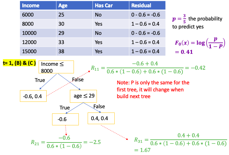
\[\begin{aligned} \color{fuchsia}{a} & = \color{fuchsia}{ \frac{1}{m} \sum_{i=1}^m y_i } \\ &= {\frac{\text{Number of Positive Class}}{\text{Total Number of Sample}}} = \color{blue}{p} \text{ probability of predicted positive} \end{aligned}\] \[F_0\left( x \right) = log\left( \frac{a}{1-a} \right) = \color{blue}{log \left( \frac{p}{1-p} \right)}\]

Note: p is only the same for the first tree. It will change when build next tree

(A): $r_{it}$: t-th tree’s i-th sample Pseudo Residuals

for i = 1, … , m is to calculate residual for all the samples in the dataset

For above,

\[- \frac{\partial L \left( y_i, F\left( x_i \right) \right)}{\partial F\left( x_i \right)} = a - y_i = \frac{1}{1+e^{-F\left( x \right)} } - y_i\\\]

When t = 1, $ F_0\left( x \right) = log \left( \frac{p}{1-p} \right) $

\[\begin{aligned} - \frac{\partial L \left( y_i, F\left( x_i \right) \right)}{\partial F\left( x_i \right)} &= \frac{1}{1+e^{-F\left( x \right)} } - y_i\\ &= \frac{1}{1+e^{-log \left( \frac{p}{1-p} \right) } } - y_i \\ &= \frac{1}{1+ \frac{1-p}{p} } - y_i \\ & = p - y_i = \color{fuchsia}{pseudo-residual} \\ \end{aligned}\]

(C): Use Talyer Series to approximate the formula, check here

\[\text{For j = 1 ... L compute } \color{Fuchsia}{r_{jt} = argmin_\gamma \sum_{x_i \in R_{jt}} L \left( y_i, F_{t-1}\left( x_i \right) + \gamma \right)} \\ \quad \color{grey}{\text{( L is total number of leaves in t-th tree )}}\] \[\sum_{x_i \in R_{jt}} L\left(y_i, F_{t-1}\left(x_i\right) + \gamma \right) \approx \sum_{x_i \in R_{jt}}L\left(y_i, F_{t-1}\left(x_i\right) \right) + \sum_{x_i \in R_{jt}}\frac{d}{d F_{t-1}\left(x_i \right)}L\left(y_i, F_{t-1}\left(x_i\right) \right)\gamma \\ + \sum_{x_i \in R_{jt}}\frac{1}{2}\frac{d^2}{d F_{t-1}\left(x_i \right)^2}L\left(y_i, F_{t-1}\left(x_i\right) \right)\gamma^2\]

As we know,

\[\begin{aligned} \text{let } p_t\left(x_i \right) &= \frac{1}{1 + e^{-F_t\left(x\right)}} \\ \frac{da}{dF_t\left( x \right)} &= p_t\left(x_i \right) * \left( 1- p_t\left(x_i \right) \right) \\ \frac{d L \left( y,F_t\left(x \right)\right)}{dF_t\left( x\right)} &= \ \sum_{i=1}^m\left( p_t\left(x_i \right) - y_i \right) = -\sum_{i=1}^m \text{pseudo-residual} \\ & \quad \color{grey}{\text{ p is the probability of predict positive}}\\ \frac{d^2 L \left( y,F_t\left(x \right)\right)}{dF_t\left( x\right)^2} &= \frac{d}{dF_t\left( x\right)} \sum_{i=1}^m\left( p_t\left(x_i \right) - y_i \right) = \frac{d}{dF_t\left( x\right)} \sum_{i=1}^m\left( \frac{1}{1+e^{-F_t\left( x\right)}} - y_i \right) \\ & = \sum_{i=1}^m\left( p_t\left(x_i \right)*(1-p_t\left(x_i \right)) \right) \end{aligned}\]

Take the derivative to $gamma$ on both side

\[\begin{aligned} \sum_{x_i \in R_{jt}}\frac{d}{d\gamma}L\left(y_i, F_{t-1}\left(x_i\right) + \gamma \right) &\approx \sum_{x_i \in R_{jt}} \frac{d}{d\gamma} L\left(y_i, F_{t-1}\left(x_i\right) \right) + \sum_{x_i \in R_{jt}}\frac{d}{d\gamma} \frac{d}{d F_{t-1}\left(x_i \right)}L\left(y_i, F_{t-1}\left(x_i\right) \right)\gamma \\ & \quad \quad +\sum_{x_i \in R_{jt}} \frac{1}{2}\frac{d}{d\gamma} \frac{d^2}{d F_{t-1}\left(x_i \right)^2}L\left(y_i, F_{t-1}\left(x_i\right) \right)\gamma^2 \\ &= 0 + \sum_{x_i \in R_{jt}}\frac{d}{d F_{t-1}\left(x_i \right)}L\left(y_i, F_{t-1}\left(x_i\right) \right)+ \sum_{x_i \in R_{jt}}\frac{d^2}{d F_{t-1}\left(x_i \right)^2}L\left(y_i, F_{t-1}\left(x_i\right) \right)\gamma \\ &= - \sum_{x_i \in R_{jt}} \text{pesudo-residual} + \sum_{x_i \in R_{jt}} \left( p_{t-1}\left(x_i\right) * （1-p_{t-1}\left(x_i\right)) \right) \gamma \end{aligned}\]

And set the derivative to Zero

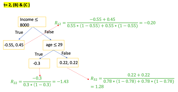
\[\gamma = \frac{\sum_{x_i \in R_{jt}} \text{pesudo-residual} }{\sum_{x_i \in R_{jt}} \left[ p_{t-1}\left(x_i\right) * （1-p_{t-1}\left(x_i\right)) \right] } = \frac{\sum_{\color{red}{leaf}} \text{residual} }{\sum_{\color{red}{leaf}} \left[ p_{t-1}\left(x_i\right) * （1-p_{t-1}\left(x_i\right)) \right] }\]

E.g. use people’s income and age to predict if the person has car

XGBoost

Note: XGBoost is designed for large, complicated data sets
The default of level of trees is 6
Regardless of classification or regression, default probability is 0.5at the first step
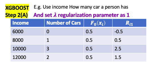
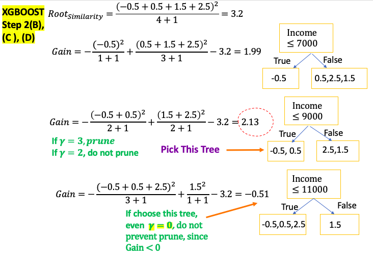
$\lambda$ is regularization parameter. it is intended to reduce the prediction’s sensitivity to individual observation** by pruning and combine them with other observations
- if $\lambda > 0$, similarity scores are smaller. The amount of decrease is inversely proportional to the number of Residuals in the node
  - e.g. only 1 residual in the leaf, $\lambda = 1$, reduce similarity by 50%
  - e.g. only 4 residual in the leaf, $\lambda = 1$, reduce similarity by 20%
- if $\lambda > 0$, it results in more pruning, by shrinking the Similarity Scores, smaller Output Values for leave, and result lower value for Gain
- when $\lambda > 0$, it reduces the amount that single observatin adds to the new prediction
- set $\lambda = 0$, doesn’t prevent tree from pruning, because $Gain < 0$, $Gain - \gamma = Gain $ still can be a negative number, so remove the branch and make it as leaf
- setting $\lambda = 1$, prevent overfitting the Training Data
XGBoost learning rate $\eta$ (eta) default value is 0.3

\[\color{red}{\text{Leaf Output Value for Regression }} = \frac{\color{fuchsia}{\text{Sum of Residuals}}}{\text{Number of Residuals } + \lambda }\] \[\color{red}{\text{Leaf Output Value for Classification }} = \color{fuchsia}{\frac{\text{Sum of Residuals}}{\sum_{x_i \in R_{jt}} \left[ p_{t-1}\left(x_i\right) * \left( 1- p_{t-1}\left(x_i\right) \right) \right] + \lambda}}\]

Similarity Score: multiply -2 to loss function when plug in $r_{jt}$ and remove the constant term (which is not link the leaf output value)

Loss function is minimize when $r_{jt} = \color{fushsia}{\text{leaf output value}}$, so negative loss function is maximize at the same point

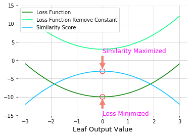
\[\begin{aligned} \sum_{x_i \in R_{jt}} \left[ L \left( y_i, F_{t-1}\left( x_i \right) + r_{jt} \right)\right] + \gamma T + \frac{1}{2} \lambda r_{jt}^2 &\approx \underbrace{\sum_{x_i \in R_{jt}}L\left(y_i, F_{t-1}\left(x_i\right) \right)}_{\color{red}{\text{constant term}}} + \sum_{x_i \in R_{jt}}\frac{d}{d F_{t-1}\left(x_i \right)}L\left(y_i, F_{t-1}\left(x_i\right) \right)r_{jt}\\ &+ \sum_{x_i \in R_{jt}}\frac{1}{2}\frac{d^2}{d F_{t-1}\left(x_i \right)^2}L\left(y_i, F_{t-1}\left(x_i\right) \right)r_{jt}^2 + \underbrace{\gamma T}_{\color{red}{\text{constant term}}} + \frac{1}{2} \lambda r_{jt}^2 \end{aligned}\]

By removing the constant term and multiply by -2

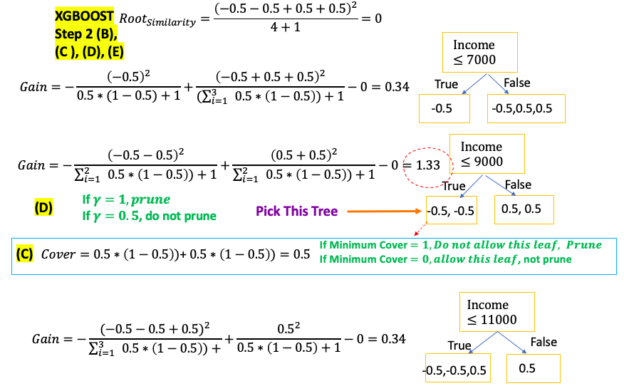
\[\text{Similarity Score} = -2\left( \sum_{x_i \in R_{jt}}\frac{d}{d F_{t-1}\left(x_i \right)}L\left(y_i, F_{t-1}\left(x_i\right) \right)r_{jt} + \sum_{x_i \in R_{jt}}\frac{1}{2}\frac{d^2}{d F_{t-1}\left(x_i \right)^2}L\left(y_i, F_{t-1}\left(x_i\right) \right)r_{jt}^2 + \frac{1}{2} \lambda r_{jt}^2 \right)\] \[\color{red}{\text{Similarity Score for Regression }} = \frac{\color{fuchsia}{\text{Squared of Sum of Residuals }}}{\text{Number of Residuals } + \lambda }\] \[\color{red}{\text{Similarity Score for Classification }} = \frac{\color{fuchsia}{\left( \sum Residual_i \right)^2}}{ \sum \left[ \text{Previous Probability}_i \times \left(1 - \text{Previous Probability}_i \right) \right] + \color{red}{\lambda} }\]

Gain: If Gain is less than $\gamma$, remove the branch. Done the pruning. Otherwise keep the branch and continue pruning

$\gamma$: user defined Tree Complexity Parameter
Prune the tree from bottom to top. If child nodes Gain is bigger than $\gamma$, done the prune even if parent nodes Gain maybe less than $\gamma$

\[Gain = Left_{Similarity} + Right_{Similarity} - \underbrace{Root_{Similarity}}_{\text{Similarity Score without branch }}\] \[Gain - \gamma = \begin{cases} > 0 & \text{do not prune} \\ < 0 & \text{prune} \\ \end{cases}\]

Then calculate the Output Values for the remaining leaves

\[\text{Leaf Output Value} = \frac{\color{fuchsia}{\text{Sum of Residuals}}}{\text{Number of Residuals } + \color{red}{\lambda }}\]

Cover:

The minimum number of Residuals in each leaf is determined by Cover (The denominator of Similarity minus $\lambda$)</span>
- Default, the minimum value for Cover is 1. In XGBoost for Regression, can have as few as 1 Residual per leaf. So Cover has no effect how we grow the tree
- For XGBoost for Classification, Cover depends on previously predicted probability of each Residual in a leaf
  - e.g. Previous Probability = 0.5, Cover = 0.5*(1-0.5) = 0.25. Since if minimum default probability = 1, will not allow this leaf

Cover is the sum of the Hessians(second derivative)(because it is the denominator of Similarity minus $\lambda$), For the detials of derivation see XGBoost for Regression $r_{jt}$

\[Cover = \sum_{x_i \in R_{jt}}\frac{d^2}{d F_{t-1}\left(x_i \right)^2}L\left(y_i, F_{t-1}\left(x_i\right) \right)\]

For Regression:

\[Cover = \text{Number of Residuals }\]

For classification:

\[Cover = \sum \left[ \text{Previous Probability}_i \times \left(1 - \text{Previous Probability}_i \right) \right]\]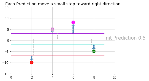

XGBoost can speed up building trees by only looking at a random subset of data (比如总共100 个observations, 只用60个 to build the tree)
XGBoost can speed up building trees by only looking at a random subset of features when deciding how to split the data (比如total 6 features, when select nodes, only look at 4 features)

XGBoost for Regression

Algorithm

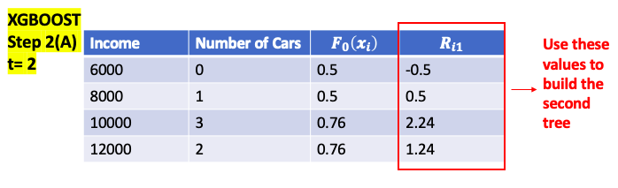
\[\begin{aligned} \text{Step 1: } & \text{ Initial Predict } = 0.5 \color{grey}{\text{ (0.5 for both regression and classification)}} \\ \text{Step 2: } & \text{ for t = 1 to T:} \color{grey}{\text{ (T is the number of Trees)}} \\ & \left(A \right) \text{Compute } \color{blue}{Residual} \text{ for i = 1...M} \color{grey}{\text{( M is the number of data)}} \\ & \quad \color{fuchsia}{r_it = y_i - F_{it}\left( x_i \right)} \\ & \left(B \right) \text{Calculate } \color{blue}{Gain} \text{ value for different combination of thresholds} \\ & \quad \color{fuchsia}{Gain = Left_{Similarity} + Right_{Similarity} - Root_{Similarity}}\\ & \quad \text{pick the one with the largest } \color{blue}{Gain}\text{ as node}\\ & \left( C \right): \text{Repeat step B till build the entire tree} \\ & \left( D \right): \text{from bottom of the tree to compare } \color{blue}{\text{ Gain with } \gamma \text{ to prune the tree }}\\ & \quad \color{fuchsia}{ Gain - \gamma = \begin{cases} > 0 & \text{do not prune} \\ < 0 & \text{prune} \\ \end{cases}} \\ & \left( E\right): \text{Compute each leaf output value for j = 1 ... L } \color{grey}{\text{( L is the total number of leaves in t-th tree)}} \\ & \quad \color{fuchsia}{r_{jt} = \frac{\text{Sum of Residuals}}{\text{Number of Residuals} + \lambda}} \\ & \left(F \right) \text{update the model, } \nu \text{ is learning rate} \\ & \quad \color{Turquoise}{F_t\left( x \right) = F_{t-1}\left( x \right) + \nu \sum_{j}^L r_{jt} I\left( x \in R_{jt} \right)} \\ \end{aligned}\]

When build the new Tree at step t, for a single leaf goal is to find an leaf Output value $r_{jt}$ minimize below equation

\[\begin{aligned} min & \sum_{x_i \in R_{jt}} \left[ L \left( y_i, F_{t-1}\left( x_i \right) + r_{jt} \right)\right] + \gamma T + \frac{1}{2} \lambda r_{jt}^2 \\ \color{red}{T } & \color{blue}{\text{ is the number of terminal nodes / leaves in a tree } } \\ \color{red}{\gamma } & \color{blue}{\text{ user definable penalty to encourage pruning } } \\ \color{red}{F_{t-1}\left( x_i \right)} & \color{blue}{\text{ previous predicted value } } \\ \color{red}{ r_{jt} } & \color{blue}{\text{ jth Leaf output value for new(t-th) built tree } } \\ \end{aligned}\] \[L\left( y_i, F_{t-1} \left( x_i \right) \right) = \frac{1}{2} \left( y_i - F_{t-1} \left( x_i \right) \right)^2\]

Can use Tayler Series to approximate the first term

\[\sum_{x_i \in R_{jt}} \left[ L \left( y_i, F_{t-1}\left( x_i \right) + r_{jt} \right)\right]\approx \sum_{x_i \in R_{jt}}L\left(y_i, F_{t-1}\left(x_i\right) \right) + \sum_{x_i \in R_{jt}}\frac{d}{d F_{t-1}\left(x_i \right)}L\left(y_i, F_{t-1}\left(x_i\right) \right)r_{jt}\\ + \sum_{x_i \in R_{jt}}\frac{1}{2}\frac{d^2}{d F_{t-1}\left(x_i \right)^2}L\left(y_i, F_{t-1}\left(x_i\right) \right)r_{jt}^2\]

So,

\[\begin{aligned} \sum_{x_i \in R_{jt}} \left[ L \left( y_i, F_{t-1}\left( x_i \right) + r_{jt} \right)\right] + \gamma T + \frac{1}{2} \lambda r_{jt}^2 &\approx \sum_{x_i \in R_{jt}}L\left(y_i, F_{t-1}\left(x_i\right) \right) + \sum_{x_i \in R_{jt}}\frac{d}{d F_{t-1}\left(x_i \right)}L\left(y_i, F_{t-1}\left(x_i\right) \right)r_{jt}\\ &+ \sum_{x_i \in R_{jt}}\frac{1}{2}\frac{d^2}{d F_{t-1}\left(x_i \right)^2}L\left(y_i, F_{t-1}\left(x_i\right) \right)r_{jt}^2 + \gamma T + \frac{1}{2} \lambda r_{jt}^2 \end{aligned}\]

Take the derivate to $r_{jt}$ on both side, check detailed derivative derivation

\[\begin{aligned} \frac{d}{d r_{jt}}\sum_{x_i \in R_{jt}} \left[ L \left( y_i, F_{t-1}\left( x_i \right) + r_{jt} \right)\right] + \gamma T + \frac{1}{2} \lambda r_{jt}^2 &\approx \frac{d}{d r_{jt}}\sum_{x_i \in R_{jt}}L\left(y_i, F_{t-1}\left(x_i\right) \right) \\ &+ \frac{d}{d r_{jt}} \sum_{x_i \in R_{jt}}\frac{d}{d F_{t-1}\left(x_i \right)}L\left(y_i, F_{t-1}\left(x_i\right) \right)r_{jt}\\ &+ \frac{d}{d r_{jt}} \sum_{x_i \in R_{jt}}\frac{1}{2}\frac{d^2}{d F_{t-1}\left(x_i \right)^2}L\left(y_i, F_{t-1}\left(x_i\right) \right)r_{jt}^2 \\ & + \frac{d}{d r_{jt}} \gamma T + \frac{d}{d r_{jt}} \frac{1}{2} \lambda r_{jt}^2 \\ & = 0 + -\sum_{x_i \in R_{jt}} \left( y_i - F_{t-1}\left( x_i\right) \right) + \sum_{x_i \in R_{jt}} \left( 1 \right) r_{jt} + 0 + \lambda r_{jt}\\ & = -\sum_{x_i \in R_{jt}} \left( \color{fuchsia}{Residuals} \right) + \color{fuchsia}{\text{Number of Residuals }r_{jt} } + \lambda r_{jt} \end{aligned}\]

Then set it to 0, can get leaf output value

\[r_{jt} = \color{fuchsia}{\frac{\text{Sum of Residuals}}{\text{Number of Residuals} + \lambda}}\]

To calculate Similarity Score

Example:

XGBoost for Clasification

Algorithm

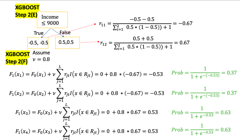
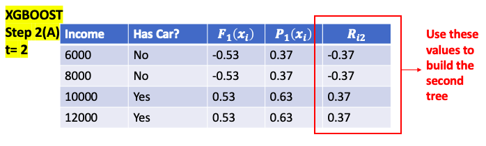
\[\begin{aligned} \text{Step 1: } & \text{ Initial Predict probability} = 0.5, \color{grey}{\text{ (0.5 for both regression and classification)}} \\ &\quad F_0\left( x_i \right) = log\left( odd \right) = log \left( \frac{0.5}{1-0.5} \right) = 0 \\ \text{Step 2: } & \text{ for t = 1 to T:} \color{grey}{\text{ (T is the number of Trees)}} \\ & \left(A \right) \text{Compute } \color{blue}{Residual} \text{ for i = 1...M} \color{grey}{\text{( M is the number of data)}} \\ & \quad \color{fuchsia}{r_it = y_i - \frac{1}{1 + e ^{-F_{t-1}\left( x \right)}}} \\ & \left(B \right) \text{Calculate } \color{blue}{Gain} \text{ value for different combination of threshold} \\ & \quad \color{fuchsia}{Gain = Left_{Similarity} + Right_{Similarity} - Root_{Similarity}}\\ & \quad \text{pick the one with the largest } \color{blue}{Gain}\text{ as node}\\ & \left( C\right) \text{compare Cover with minimum Cover value to decide if keep the branch} \\ & \quad \color{fuchsia}{Cover = \sum_{x_i \in R_{jt}} \left[ p_{t-1}\left(x_i\right) * \left( 1- p_{t-1}\left(x_i\right) \right) \right]} \\ & \color{YellowGreen}{\quad = \begin{cases} > \text{Minimum Cover} & \text{do not prune} \\ < \text{Minimum Cover} & \text{prune} \\ \end{cases}} \\ & \left( D \right): \text{Repeat step B and C till build the entire tree} \\ & \left( E \right): \text{from bottom of the tree to compare } \color{blue}{\text{ Gain with } \gamma \text{ to prune the tree }}\\ & \quad \color{YellowGreen}{ Gain - \gamma = \begin{cases} > 0 & \text{do not prune} \\ < 0 & \text{prune} \\ \end{cases}} \\ & \left( F\right): \text{Compute each leaf output value for j = 1 ... L } \color{grey}{\text{( L is the total number of leaves in t-th tree)}} \\ & \quad \color{fuchsia}{r_{jt} = \frac{\text{Sum of Residuals}}{\sum_{x_i \in R_{jt}} \left[ p_{t-1}\left(x_i\right) * \left( 1- p_{t-1}\left(x_i\right) \right) \right] + \lambda}} \\ & \left(G \right) \text{update the model, } \nu \text{ is learning rate} \\ & \quad \color{Turquoise}{F_t\left( x \right) = F_{t-1}\left( x \right) + \nu \sum_{j}^L r_{jt} I \left( x \in R_{jt} \right)} \\ \text{Step 3: } & \text{ Convert log(odds) to Probability } \\ & \quad \color{Turquoise}{ Prediction = \frac{1}{1 + e ^{-F_T\left( x \right)}}}\\ \end{aligned}\]

When build the new Tree at step t, for a single leaf goal is to find an leaf Output value $r_{jt}$ minimize below equation

\[\begin{aligned} min & \sum_{x_i \in R_{jt}} \left[ L \left( y_i, F_{t-1}\left( x_i \right) + r_{jt} \right)\right] + \gamma T + \frac{1}{2} \lambda r_{jt}^2 \\ \color{red}{T } & \color{blue}{\text{ is the number of terminal nodes / leaves in a tree } } \\ \color{red}{\gamma } & \color{blue}{\text{ user definable penalty to encourage pruning } } \\ \color{red}{F_{t-1}\left( x_i \right)} & \color{blue}{\text{ previous predicted value } } \\ \color{red}{ r_{jt} } & \color{blue}{\text{ jth Leaf output value for new(t-th) built tree } } \\ \end{aligned}\] \[L \left( y_i, F_{t-1}\left( x_i \right) \right) = - y_i log \left( \frac{1}{1+ e^{-F_{t-1}\left( x_i \right)}} \right) + (1-y_i) log \left( 1- \frac{1}{1+ e^{-F_{t-1}\left( x_i \right)}} \right)\]

Can use Tayler Series to approximate

\[\begin{aligned} \sum_{x_i \in R_{jt}} \left[ L \left( y_i, F_{t-1}\left( x_i \right) + r_{jt} \right)\right] + \gamma T + \frac{1}{2} \lambda r_{jt}^2 &\approx \sum_{x_i \in R_{jt}}L\left(y_i, F_{t-1}\left(x_i\right) \right) + \sum_{x_i \in R_{jt}}\frac{d}{d F_{t-1}\left(x_i \right)}L\left(y_i, F_{t-1}\left(x_i\right) \right)r_{jt} \\ &+ \sum_{x_i \in R_{jt}}\frac{1}{2}\frac{d^2}{d F_{t-1}\left(x_i \right)^2}L\left(y_i, F_{t-1}\left(x_i\right) \right)r_{jt}^2 + \gamma T + \frac{1}{2} \lambda r_{jt}^2 \end{aligned}\]

Take the derivate to $r_{jt}$ on both side, check detailed derivative derivation

\[\begin{aligned} \frac{d}{d r_{jt}}\sum_{x_i \in R_{jt}} \left[ L \left( y_i, F_{t-1}\left( x_i \right) + r_{jt} \right)\right] + \gamma T + \frac{1}{2} \lambda r_{jt}^2 &\approx \frac{d}{d r_{jt}}\sum_{x_i \in R_{jt}}L\left(y_i, F_{t-1}\left(x_i\right) \right) \\ &+ \frac{d}{d r_{jt}} \sum_{x_i \in R_{jt}}\frac{d}{d F_{t-1}\left(x_i \right)}L\left(y_i, F_{t-1}\left(x_i\right) \right)r_{jt} \\ &+ \frac{d}{d r_{jt}} \sum_{x_i \in R_{jt}}\frac{1}{2}\frac{d^2}{d F_{t-1}\left(x_i \right)^2}L\left(y_i, F_{t-1}\left(x_i\right) \right)r_{jt}^2 \\ & + \frac{d}{d r_{jt}} \gamma T + \frac{d}{d r_{jt}} \frac{1}{2} \lambda r_{jt}^2 \\ & = 0 + -\sum_{x_i \in R_{jt}} \left( p_{t-1}\left(x_i\right) - F_{t-1}\left( x_i\right) \right) \\ & + \sum_{x_i \in R_{jt}} \left( p_{t-1}\left(x_i\right) * \left( 1- p_{t-1}\left(x_i\right) \right) \right) r_{jt} + 0 + \lambda r_{jt}\\ &\color{blue} {Note: p_{t-1}\left(x_i\right) = \frac{1}{1 + e^{- F_{t-1}\left(x_i \right)}}, F_{t-1}\left(x_i \right) = log\left( \frac{p_{t-1}\left(x_i\right)}{1- p_{t-1}\left(x_i\right)} \right) } \\ & = -\sum_{x_i \in R_{jt}} \left( \color{fuchsia}{Residuals} \right) + \color{fuchsia}{ \sum_{x_i \in R_{jt}} \left[ p_{t-1}\left(x_i\right) * \left( 1- p_{t-1}\left(x_i\right) \right) \right] r_{jt} } + \lambda r_{jt} \end{aligned}\]

Then set it to 0, can get leaf output value

\[r_{jt} = \color{fuchsia}{\frac{\text{Sum of Residuals}}{\sum_{x_i \in R_{jt}} \left[ p_{t-1}\left(x_i\right) * \left( 1- p_{t-1}\left(x_i\right) \right) \right] + \lambda}}\]

Calculate the Similarity Score:

\[\begin{aligned} \text{Similarity Score} &= -2\left( \sum_{x_i \in R_{jt}}\frac{d}{d F_{t-1}\left(x_i \right)}L\left(y_i, F_{t-1}\left(x_i\right) \right)r_{jt} + \sum_{x_i \in R_{jt}}\frac{1}{2}\frac{d^2}{d F_{t-1}\left(x_i \right)^2}L\left(y_i, F_{t-1}\left(x_i\right) \right)r_{jt}^2 + \frac{1}{2} \lambda r_{jt}^2 \right)\\ &= -2 \left(-\sum_{x_i \in R_{jt}} \color{blue}{Residuals } \right) r_{jt} - \color{blue}{ \sum_{x_i \in R_{jt}} \left[ p_{t-1}\left(x_i\right) * \left( 1- p_{t-1}\left(x_i\right) \right) \right] }r_{jt}^2 - \lambda r_{jt}^2 \\ &= 2\left( \color{blue}{\text{ Sum of Residuals } } \right) r_{jt} - \left(\color{blue}{ \sum_{x_i \in R_{jt}} \left[ p_{t-1}\left(x_i\right) * \left( 1- p_{t-1}\left(x_i\right) \right) \right] } + \lambda\right) r_{jt}^2 \\ &\color{grey}{\text{Then plug in } r_{jt}}= \color{Tan}{\frac{\text{Sum of Residuals}}{\sum_{x_i \in R_{jt}} \left[ p_{t-1}\left(x_i\right) * \left( 1- p_{t-1}\left(x_i\right) \right) \right] + \lambda}} \\ &=2\left( \color{blue}{\text{ Sum of Residuals } } \right) \color{Tan}{\frac{\text{Sum of Residuals}}{\sum_{x_i \in R_{jt}} \left[ p_{t-1}\left(x_i\right) * \left( 1- p_{t-1}\left(x_i\right) \right) \right] + \lambda}} \\ & - \left(\color{blue}{\text{Number of Residuals } } + \lambda\right) \left(\color{Tan}{\frac{\text{Sum of Residuals}}{\sum_{x_i \in R_{jt}} \left[ p_{t-1}\left(x_i\right) * \left( 1- p_{t-1}\left(x_i\right) \right) \right] + \lambda}} \right)^2 \\ &= 2 \color{black}{\frac{\text{( Sum of Residuals )}^2}{\sum_{x_i \in R_{jt}} \left[ p_{t-1}\left(x_i\right) * \left( 1- p_{t-1}\left(x_i\right) \right) \right] + \lambda}} - \color{black}{\frac{\text{( Sum of Residuals )}^2}{\sum_{x_i \in R_{jt}} \left[ p_{t-1}\left(x_i\right) * \left( 1- p_{t-1}\left(x_i\right) \right) \right] + \lambda}} \\ &= \color{fuchsia}{\frac{\text{( Sum of Residuals )}^2}{\sum_{x_i \in R_{jt}} \left[ p_{t-1}\left(x_i\right) * \left( 1- p_{t-1}\left(x_i\right) \right) \right] + \lambda}} \end{aligned}\]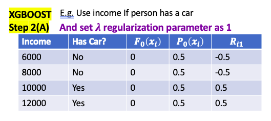

Approximate Greedy Algorithm

XGBoost use Greedy algorithms to select threshold with the largest gain
- Note: use the theshold that gives largest Gain is made without worrying about how the leaves will be split later
- Use Greey Algorithm without look the absolute best choice in the long term. So it can build a tree relatively quickly
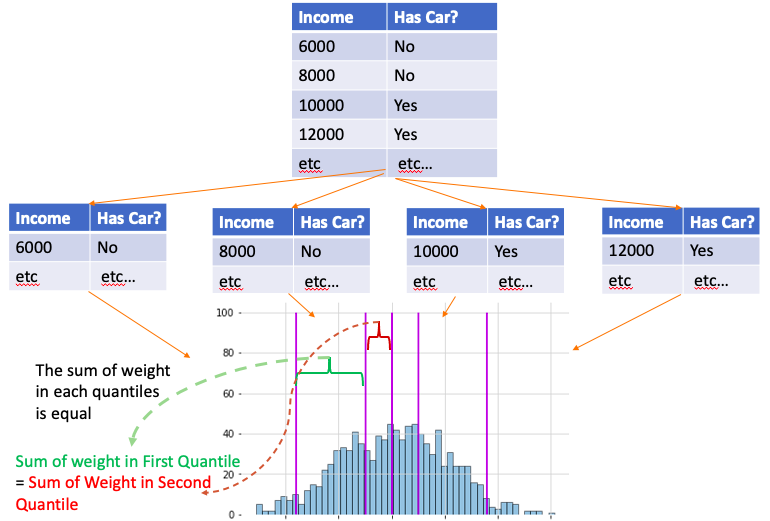
For large dataset, it is slow because looking at every possible threshold for every single variable, e.g. 1M data with 6 variable, total check (1M-1)*6
Approximate Greedy Algorithm: instead of testing every single threshold, could divide data into Quantiles and use the Quantiles as candidate threshold to split the observations
- More Quantile -> More Accurate -> More time to test and build the tree
- Default for Approximate Greedy Algorithm use 33 Quantiles

Weighted Sketch Algorithm

can’t fit all data into computer’s memory at one time, and sorting number, finding quantile become really slow
Splitting data into different pieces on different computers on a network
- Using Parallel Learning so that multiple computers can work at the same time
Quantile Sketch Algorithm combines values from each computer to make an approximate histogram
Then approximate histogram is used to calculate approximate quantiles and approximate Greedy Algorithm use approximate quantiles
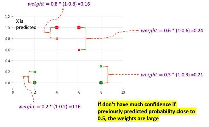
Each observation has a corresponding weight, and the sum of weight is equal in each quantile
- For classification: The weight is derived from Cover Metrics (2nd derivative of the Loss function, Hessian): $P_{t-1}\left(x_i\right)* \left(1- P_{t-1}\left(x_i\right) \right) $
- For Regression, the weight is 1. It means weighted quantiles just like normal quantiles and contain an equal number of observations
- If don’t have much confidence if previously predicted probability close to 0.5, the weights are large
Treat each quantile as a unit, so sample within the same quantile will end up to same leaf together
- By dividing the observations into quantiles where sum of the weights are similar, put observations with low confidence predictions into quantitles with fewer observations
XGBoost only use Approximate Greedy Algorithm, Parallel Learning and Weighted Quantile Sketch when the training Data is huge
- if training data is small, just use

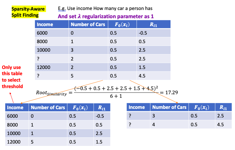
Sparsity-Aware Split Finding

Have missing value for features for training data. Even if feature value is missing, can calculate the residual
Then split data into two groups. One with full data another is with missing data.
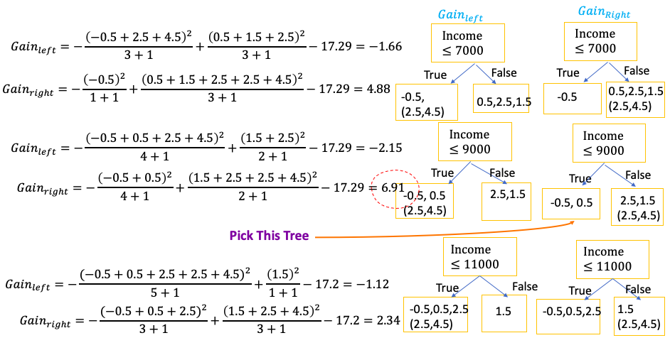
Then use full data to build the tree, and when calculate Gain and Similarity, then put the residual of missing data on left tree and right tree to calculate two Gains: $Gain_{left}$ and $Gain{right}$
Then choose the threshold which give the largest Gain
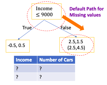
- When at evaluation, if still have missing value, the default path of missing value is the path which has the largest Gains for missing value

Does it takes much memory by doing this, since each tree Gains need to calculate twice than before?

XGBoost use Spare Matrices, it only keep track of 1s for categorical data(One Hot Vector) and deoesn’t allocate memory for zeros (Check it 35:52)

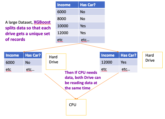
Cache-Aware Access

CPU has a small amount Cache memory(can use this memory faster than any other memory)
CPU also is attached to a large amount of Main Memory. While the Main Memory is large than the Cache, it takes longer to use
CPU also is attached to the Hard Drive. The Hard Drive can store the most stuff and slowest to use
If want program to run fast, goal is to maximize the Cache memory
XGBoost put the Gradients and Hessians(second derivatives) in the Cache so it can rapidly calculate Similarity Scores and Output Values

Blocks for Out-of-Core Computation

if dataset is too large for the Cache and Main Memory, some of it must stored on the Hard Drive
Because reading and writing data on Hard Drive is super slow, XGBoost tries to minimize these actions by compressing the data
- Even though CPU must spend some time decompressing the data that comes from the Hard Drive, it can do faster than that Hard Drive can read the data
- In other words, by spending a little bit of CPU time uncompressing the data, can avoid spending a lot of time accessing the Hard Drive
- When there is more than one Hard Drive available for storage, XGBoost uses a database technique called Sharding to speed up disk access
- It is an optimizations that take computer hardware into account

SVM

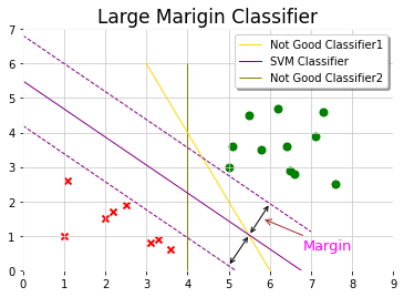
Large Margin Classifier

Cost Function

Can think of $ C \approx \frac{1}{\lambda}$

\[min_{\theta} C \sum_{i=1}^m \left[ y^{\left( i \right)} cost_1 \left( \theta^T x^{\left( i \right)}\right) + \left( 1 - y^{\left( i \right)} \right)cost_0 \left( \theta^T x^{\left( i \right)}\right)\right] + \frac{1}{2} \sum_{i=1}^n \theta_j^2\]

SVM doesn’t output probability, instead it directly predict if y is 1 or 0

\[h_\theta \left( x \right) = \begin{cases} 1 & \text{if } \theta^T x \geq 0 \\ 0 & otherwise \end{cases}\]

Support Vector Machine want to do more than that. If predict to positive, not just a little larger than 0. Or if predict to negative, not just a little smaller than 0. Maybe want to positive to bigger than 1 and negative to smaller than -1 to make cost function as 0

\[h_\theta \left( x \right) = \begin{cases} 1 & \text{if } \theta^T x \geq 1 \\ 0 & \text{if } x \leq -1 \end{cases}\]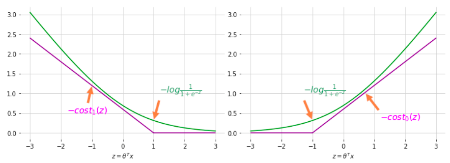

Decision Boundary

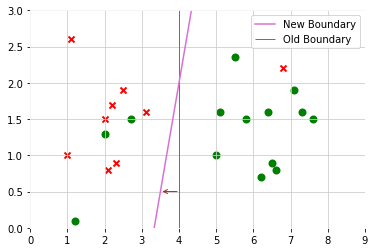
When regularization parameter C is large, SVM is very sensitive to outlier

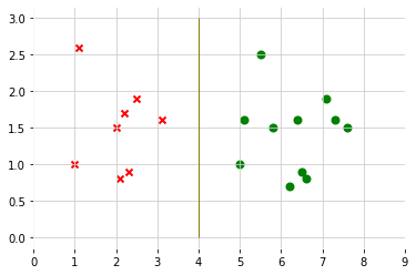
After adding a positive example, then decision boundary will change

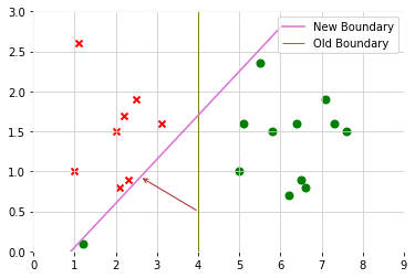
But regularization parameter C is not too large, SVM will still get the similar decision boundary to do the right thing even if data is not linearly separatable(some positive data mix in negative class, some negative data mix in positive class)

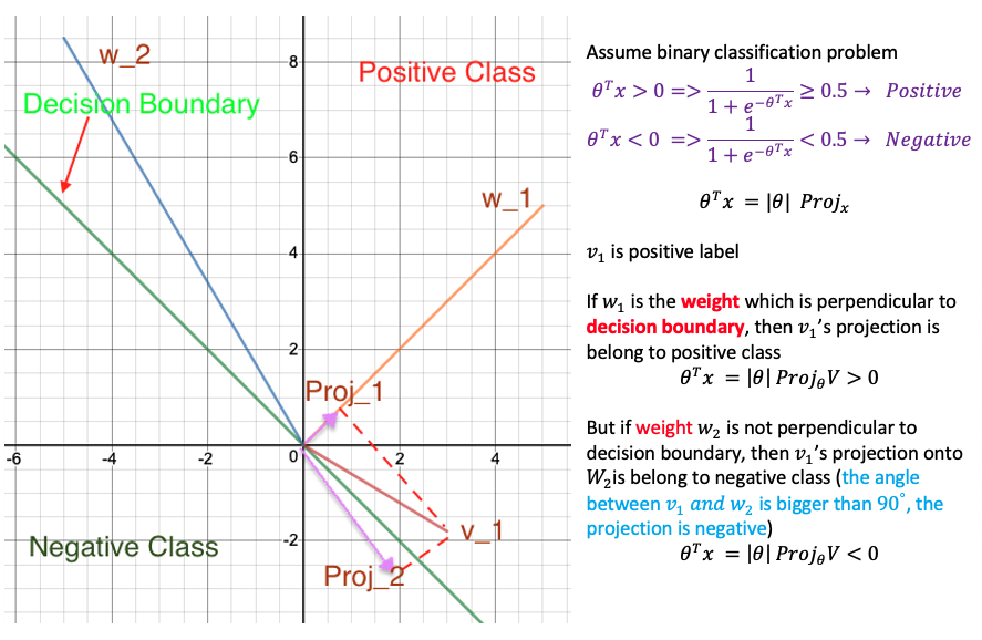
Inner Product

\[\begin{aligned} u^Tv & = u_1 v_1 + u_2 v_2 \text{ in two dimensional vector space}\\ & = \| u \| \| v\| cos \left( u, v\right) \\ & = Proj_u v \| u\| \text{ projection value can be positive or negative } \end{aligned}\] \[min_{\theta} \underbrace{C \sum_{i=1}^m \left[ y^{\left( i \right)} cost_1 \left( \theta^T x^{\left( i \right)}\right) + \left( 1 - y^{\left( i \right)} \right)cost_0 \left( \theta^T x^{\left( i \right)}\right)\right]}_{\text{set equal to 0 for perfect classification} } + \frac{1}{2} \sum_{i=1}^n \theta_j^2\]

The the cost function is

\[min_{\theta} \frac{1}{2} \sum_{i=1}^n \theta_j\] \[\begin{aligned} s.t. \quad \theta^T x^{\left( i \right)} \geq 1 & \quad \text{ if } x^{\left( i \right)} = 1 \\ \theta^T x^{\left( i \right)} \leq -1 & \quad \text{ if } x^{\left( i \right)} = 0 \\ \end{aligned}\]

assume in two dimensional space and $\theta_0 = 0$: is to minimize the square of norm/length of theta

\[min_{\theta} \frac{1}{2} \sum_{i=1}^n \theta_j = min_{\theta} \frac{1}{2}\left( \theta_1^2 + \theta_2^2 \right) = min_{\theta} \frac{1}{2}\left( \underbrace{ \sqrt{ \theta_1^2 + \theta_2^2 }}_{ \color{red}{= \| \theta \|}} \right) ^2\]

And and rewrite $\theta^T$ as projection where $ p^{\left(i \right)}$ is the projection of $x^{\left( i \right)}$ onto the vector $\theta$

\[\begin{aligned} s.t. \quad \theta^T x^{\left( i \right)} = \color{fuchsia}{ p^{\left(i \right)} \| \theta \| } \geq 1 & \quad \text{ if } x^{\left( i \right)} = 1 \\ \theta^T x^{\left( i \right)} = \color{fuchsia}{ p^{\left(i \right)} \|\theta \| } \leq -1 & \quad \text{ if } x^{\left( i \right)} = 0 \\ \end{aligned}\]

By making the margin large, can end up with smaller $\theta$ what is trying to do with the objective

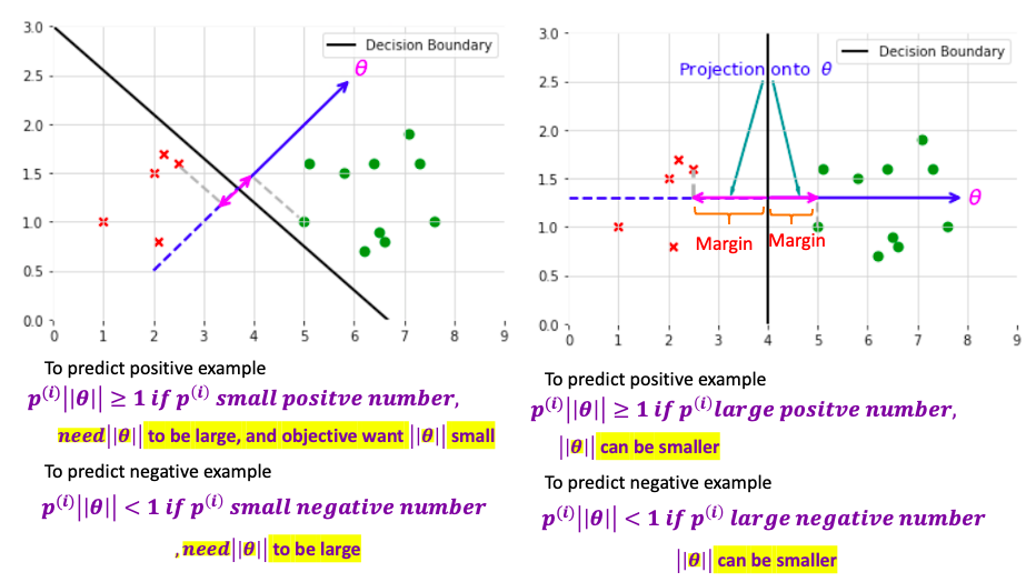
Make the whole derivation using $\theta_0 = 0$ (Decision boundary should pass the origin). When $\theta_0 \neq 0$, it also can be proved that SVM is trying to find large margin separater witht the same objective and correspond C is large

Why weight is perpendicular to decision boundary?

Gaussian Kernel

To predict y = 1 if

\[\theta_0 + \theta_1 x_1 + \theta_2 x_2 + + \theta_3 x_1 x_2 \\ + \theta_4 x_1^2 + + \theta_5 x_2^2 \cdots \geq 0\]

Can write to another representation

\[\theta_0 + \theta_1 \underbrace{f_1}_{= x_1} + \theta_2 \underbrace{f_2}_{= x_2} + \theta_3 \underbrace{f_3}_{= x_1 x_2} \\ + \theta_4 \underbrace{f_4}_{= x_1^2} + \theta_5 \underbrace{f_5}_{= x_2^2} \cdots \geq 0\]

Is there a different / better choice of features $f_1, f_2, f_3$? because above polynomials are the not the one we want

Gassian Kernel and Similarity: measure how similar vector x is from landmark

similarity between vector x and landmark $ l^{\left( 1 \right)$ (n is the number of features)

\[\color{fuchsia}{similarity\left( x, l^{\left( 1\right)}\right) = exp \left( -\frac{\| x - l^{\left( 1 \right)} \| }{2 \sigma^2}\right) = exp \left( -\frac{ \sum_{j=1}^n \| x - l_j^{\left( 1 \right)} \|}{2 \sigma^2}\right)}\]

If $x \approx l^{\left( 1 \right)}$

\[similarity\left( x, l^{\left( 1\right)}\right) = exp \left( -\frac{ 0 }{2 \sigma^2}\right) = 1\]

If x far from $ l^{\left( 1 \right)}$

\[similarity\left( x, l^{\left( 1\right)}\right) = exp \left( -\frac{ \left( \text{large number} \right)^2 }{2 \sigma^2}\right) = 0\]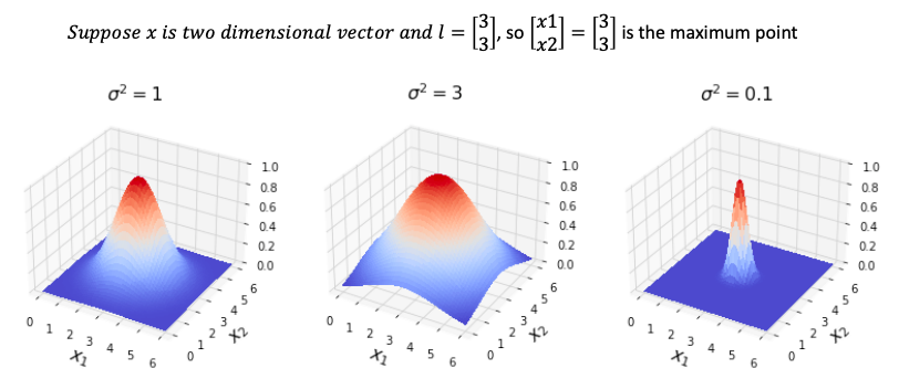

when $\sigma$ is small, the number inside exp is large, similarity fall to zero rapidly
when $\sigma$ **is **large, the number inside exp is small, similarity fall to zero slowly

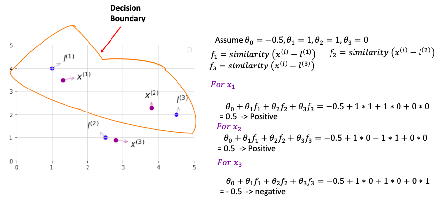
Algorithm

\[\begin{aligned} \text{Step 1}. & Given \left( x_1, y_1 \right),\left( x_2, y_2 \right), \left( x_m, y_m \right) \\ & \color{grey}{\text{suppose each x has n features ( n-dimensional)}} \\ \text{Step 2}. & \text{ choose } \color{fuchsia}{l^{\left( 1 \right)} = x_1, l^{\left( 2 \right)} = x_2, \cdots, l^{\left( m \right)} = x_m} \\ & \color{grey}{\text{(each landmark is n-dimensional )}} \\ \text{Step 3}. & \text{ for each example } x_i \\ & f^{\left( i \right)} = \begin{bmatrix} f_0^\left(i \right) \\ f_1^\left(i \right)\\ f_2^\left(i \right)\\ \vdots\\ f_m^\left(i \right)\\ \end{bmatrix} = \begin{bmatrix} \color{fuchsia}{1} \\ \color{fuchsia}{similarity\left( x^\left(i \right), l^\left(1 \right) \right)} \\ \color{fuchsia}{similarity\left( x^\left(i \right), l^\left(2 \right) \right)} \\ \color{fuchsia}{\vdots} \\ \color{fuchsia}{similarity\left( x^\left(i \right), l^\left(m \right) \right)}\\ \end{bmatrix} \\ & \color{blue}{f^{\left( i \right)} \text{ is } \left(m+1\right) \times \text{ 1 matrix } } \end{aligned}\]

Now, Cost function becomes

\[min_{\theta} C \sum_{i=1}^m \left[ y^{\left( i \right)} cost_1 \left( \theta^T \color{fuchsia}{f^{\left( i \right)}}\right) + \left( 1 - y^{\left( i \right)} \right)cost_0 \left( \theta^T \color{fuchsia}{f^{\left( i \right)}}\right)\right] + \frac{1}{2} \sum_{i=1}^n \theta_j^2\]

Another way to write $ \sum_{i=1}^n \theta_j^2$ is $\theta^T \theta$ and ignore $\theta_0$

Another way to write is $θ^T Mθ$ (M depends on the kernel you used) With the computational trick, Then computer run more efficiently for SVM using kernel, scale to much bigger training set. Logtistic regression can also use kernel function. But computational trick for SVM not work for logistic regression, it will be very slow.

Choose Parameter

can think of C as $\frac{1}{\lambda}$

Large C: low bias, high variance
Small C: high bias, low variance
Large $\sigma^2$: high bias, low variance, features $f_i$ vary more smoothly
Small $\sigma^2$: low bias, high variance, features $f_i$ vary less smoothly

Using SVM

Need to specify

Need to choose C
Need to choose kernel function

1- Linear Kernel is No Kernel: can think of special version of SVM that give standard linear classifier

use if n is big (large number of features), m is mall (small training set). You want to fit a linear decision boundardy instead to fit a complex function which may overfit because not having too much data

Predict y = 1 if $\theta^T x \geq 0$ ($\theta_0 + \theta_1 x_1 + \cdots + \theta_n x_n$)

2- Gaussian Kernel: use it when n (the number of feature) is small, m (training set) is large

Note: Do Perform Feature Scaling before using Gaussian Kernel.
- e.g. to predict housing price, $x_1$ income, $x_2$ is number of bedroom. $x_1 - l_1 = 100,000 - 50,000$ and $x_2 - l_2 = 4-1$. So similarity is dominated by the income

3- Other choice of Kernel (Kernel need to satisfy technical condition called “Mercer’s Theorem”to make sure SVM run correctly, do not diverge. Otherwise, not valid kernel). Mercer’s Theorem: What it does to assure kernel can use optimization to solve $\theta$ quickly. There are some kernels which satisfy Mercer’s Theorem but rarely to use

. Polynomial Kernel: similarity(x,l) = $\left(x^T𝐿\right)^2 or \left(x^T L \right)^3., \left(x^T L+5\right)^3, or \left(x^T L+1\right)^4$( can change what number to add and what polynomial degree). Usually work for data which are strictly non-negative. so inner product is non-negative
- Usually perform worse than Gaussian Kernel
More esoteric: String Kernel(when input are strings), Chi-square kernel, histogram intersection kernel

Many SVM packages already have built-in multi-class Classification(more than two categories) functionality OR use one vs_all method(try K SVMs, one to distinguish y=i from the rest), pick class i with largest $\left(\theta^{\left( i \right)}\right)^T x$

SVM vs Logistic Regression

Use logistic regression or SVM without a kernel,
- If n is large(feature) relative to m(training set), n>=m, e.g, n=10000, m = 10 to 1000
Use SVM with Gaussian Kernel
- If n is small, m is intermediate (n = 1-1000, m = 10-10000)
Use logistic regression or SVM without a kernel (similar performance), or add more features
- If n is small, m is large (n = 1-1000, m=50000+) Gaussian kernel is slow
Logistic Regression & SVM (numerical optimization to run faster) usually give the same performance Neural Network likely work well for most of these settings, but may be slower to train. SVM is convex optimization problem so always find the global minimum. Local minimum maybe a problem for Neural Network

References StatQuest

Random Forest, AdaBoost, Gradient Boost, XGBoost

Logit Function

Decision Tree

Regression Tree

Cost Complexity Prune Tree

Random Forest

Build Random Forest

Evaluation

Missing Values

AdaBoost

Create a Forest of Stumps using AdaBoost

Bagging Vs Boosting

Gradient Boost

Gradient Boost for Regression

Gradient Boost for Classification

XGBoost

XGBoost for Regression

XGBoost for Clasification

Approximate Greedy Algorithm

Weighted Sketch Algorithm

Sparsity-Aware Split Finding

Cache-Aware Access

Blocks for Out-of-Core Computation

SVM

Cost Function

Decision Boundary

Inner Product

Gaussian Kernel

Choose Parameter

Using SVM

SVM vs Logistic Regression

CATALOG

FEATURED TAGS