1.1 Vocabulary & Feature Extraction
Sparse Representation
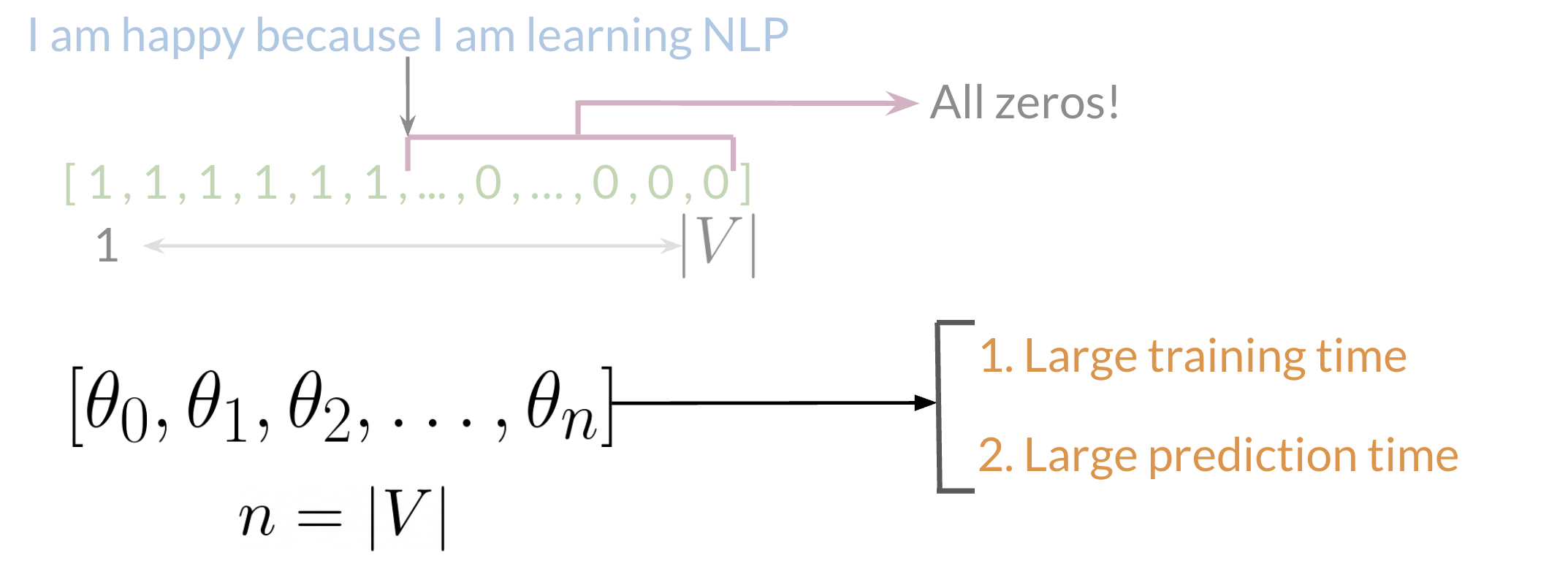
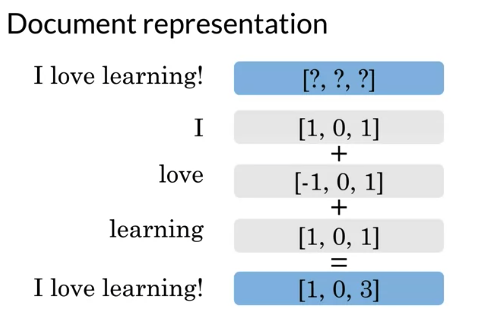
- Represent Text as a vector. Check every word from vocabulary, if appear, note 1 else 0
- Disadvantage: Large
- Logistric regression learn N+1 where N is the size of vocabulary
- Build vocabulary: process one by one and get sets of lists of word
e.g. I am happy because I am learning NLP

[I, am, happy, because, learning NLP, ... hated, the, movie]
 1   1   1       1         1       1        0     0     0
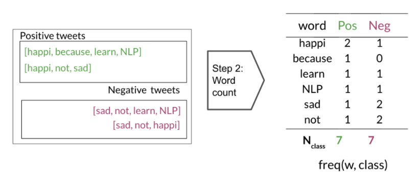
Positive & Negative Frequencies: Build vocabulary, map word to frequencey. 对所有positive examples 数vocabulary 中每个word 出现的次数, 对所有negative examples, 数vocabulary 中每个word 出现的次数
Faster speed for logistic regression, Instead learning V feature(size of vocabulary), only learn 3 features
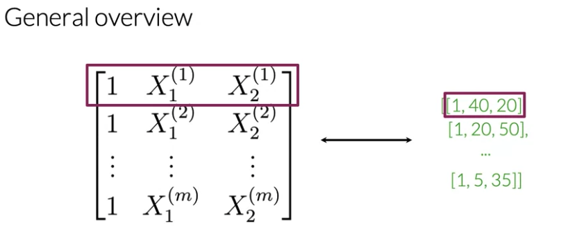
\[X_m = \left[ 1, \sum_{w_{pos}} freqs\left( w_{pos}, 1 \right), \sum_{w_{neg}} freqs\left( w_{neg}, 1 \right) \right]\]
Hence you end up getting the following feature vector [1,8,11]. 1 corresponds to the bias, 8 the positive feature, and 11 the negative feature.
Preprocessing
When preprocessing, you have to perform the following:
- Eliminate handles(@…) and URLs
- Tokenize the string into words.
- Remove stopwords like “and, is, are, at, has, for ,a”: Stop words are words that don’t add significant meaning to the text.
- Stemming- or convert every word to its stem. Like dancer, dancing, danced, becomes ‘danc’. You can use porter stemmer to take care of this.
- Convert all your words to lower case.
matrix with m rows and three columns. Every row: the feature for each tweets
General Implementation:
freqs = build_freqs(tweets,labels) #Build frequencies dictionary

X = np.zeros((m,3)) #Initialize matrix X

for i in range(m): #For every tweet

    p_tweet = process_tweet(tweets[i]) #process tweet, include

                                      # deleting stops, stemming, deleting URLS, and handles and lower cases

    X[i, :] = extract_features(p_tweet, freqs) #Extract Features:

                                               #By summing up the positive and negative frequencies of the tweets
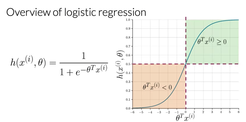
Logistic Regression
\(x^{\left( i \right)}\) is i-th tweet
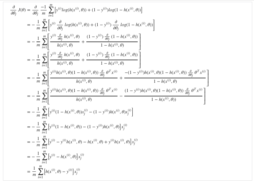
Logistic Cost Function Derivation
\[P\left( y \mid x^{\left( i \right)}, \theta \right) = h \left(x^{\left( i \right)}, \theta \right)^{y^\left( i \right)} \left( 1- h \left(x^{\left( i \right)}, \theta \right) \right)^{\left( 1- y^\left( i \right) \right)}\]when y = 1, you get \(h \left(x^{\left( i \right)}, \theta \right)\), when y = 0, you get \(\left( 1- h \left(x^{\left( i \right)}, \theta \right) \right)\). In either case, you want to maximize \(h \left(x^{\left( i \right)}, \theta \right)\) clsoe to 1. when y = 0, you want \(\left( 1- h \left(x^{\left( i \right)}, \theta \right) \right)\) to be 0 as \(h \left(x^{\left( i \right)}, \theta \right)\) close to 1, when y = 1, you want \(h \left(x^{\left( i \right)}, \theta \right) = 1\)
Define the likelihood as
\[L\left( \theta \right) = \prod_{i=1}^{m} h \left(\theta, x^{\left( i \right)} \right)^{y^\left( i \right)} \left( 1- h \left(\theta, x^{\left( i \right)} \right) \right)^{\left( 1- y^\left( i \right) \right)}\]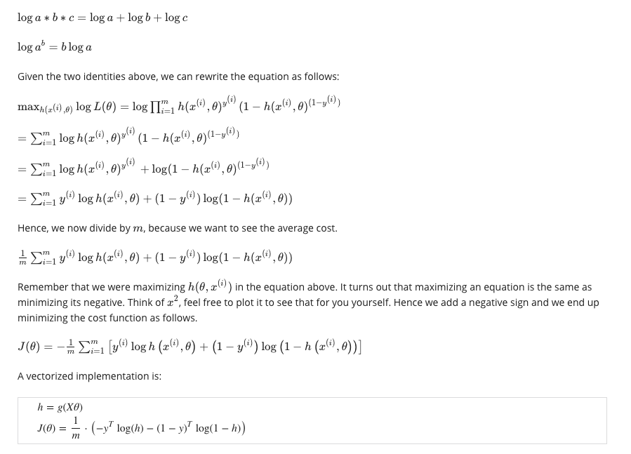
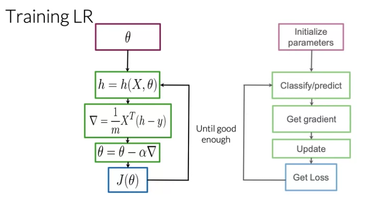
Gradient Descent Derivation
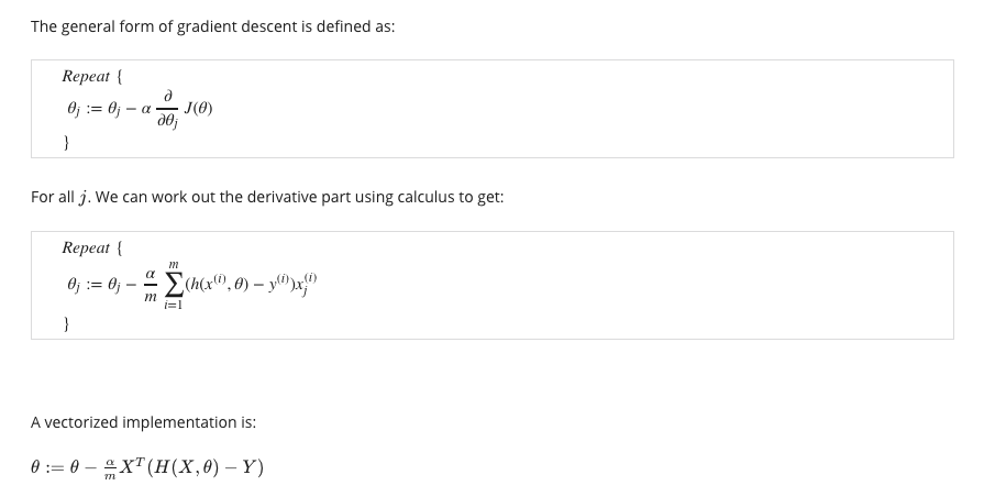
if X is M x <> matrix, N is the number of features
\[d\theta = \frac{1}{m} \left( h\left(X, \theta \right) - y \right) X^T\]if X is M x N matrix, N is the number of features
\[d\theta = \frac{1}{m} X^T \left( h\left(X, \theta \right) - y \right)\]1.2 Naive Bayes
Tweet defined either positive or negative, cannot be both. Bayes’ rule is based on the mathmatical formulation of conditional probabilities. Called Naive because make assumpton that the features you’re using for classification are all independent, which in reality is rare
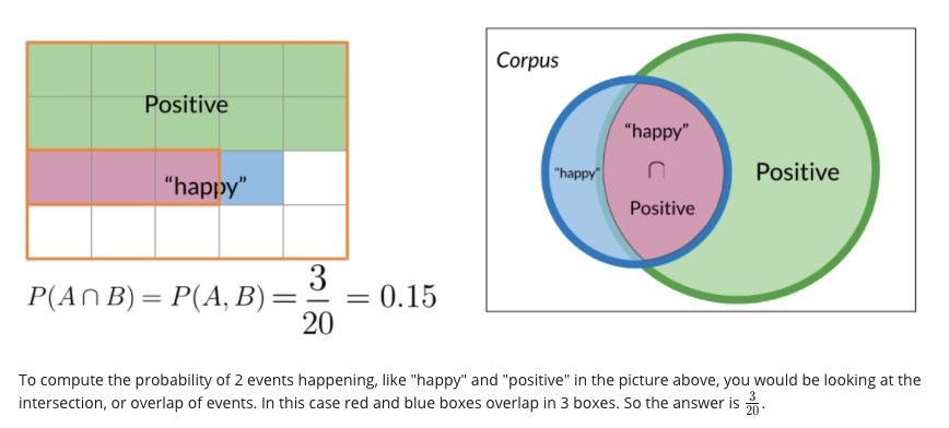
\[P\left(X \mid Y \right) = \frac{ P\left(Y \mid X \right) P\left(X \right)}{P\left(Y \right)}\]e.g. Happy sometimes as positive word sometimes as negative, A the number of positive tweet, B the number tweet contain happy
e.g. Q: Suppose that in your dataset, 25% of the positive tweets contain the word ‘happy’. You also know that a total of 13% of the tweets in your dataset contain the word ‘happy’, and that 40% of the total number of tweets are positive. You observe the tweet: ‘‘happy to learn NLP’. What is the probability that this tweet is positive?
A: 0.77
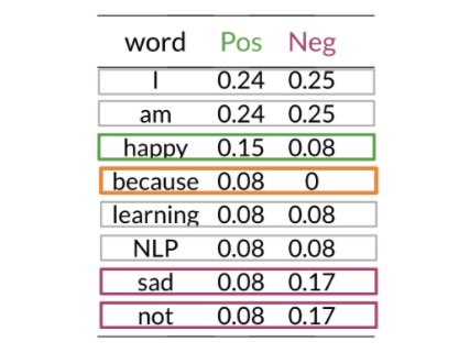
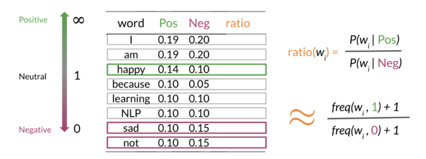
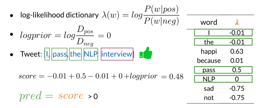
- Word with equal probability for positive/negative don’t add anything to the sentiment (e.g. I, am, learning, NLP)
- “sad, happy, not” have a significant difference between probabilities.
- Problem: “because” negative class is zero, no way of comparing between two corpora
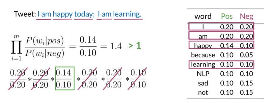
Once you have the probabilities, you can compute the likelihood score as follows. A score greater than 1 indicates that the class is positive, otherwise it is negative.
Laplacian Smoothing
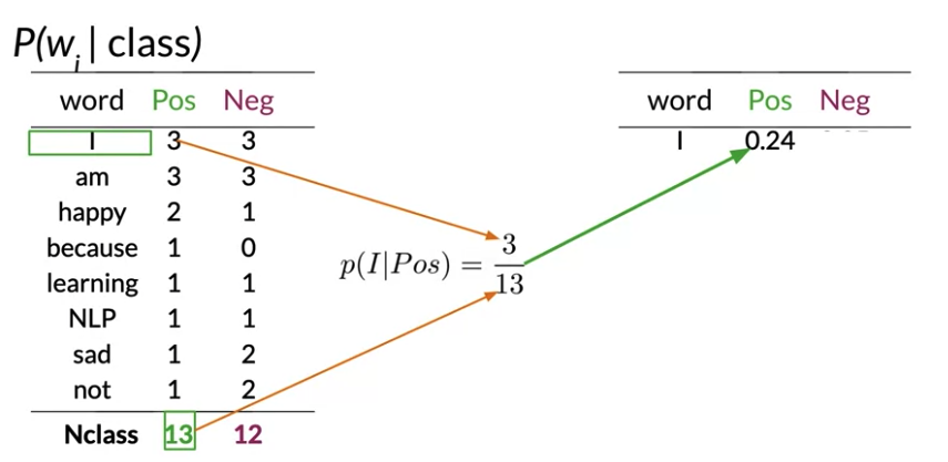
We usually compute the probability of a word given a class as follows:
\[P\left(w_i \mid class \right) = \frac{freq\left(wi,class \right)}{N_{class}} \quad \text{class} \in \text{\{Positive, Negative\}}\]- \(freq_{positive}\) and \(freq_{negative}\) are the frequencies of that specific word in the positive or negative class. In other words, the positive frequency of a word is the number of times the word is counted with the label of 1.
- \(N_{positive}\) and \(N_{negative}\) are the total number of positive and negative words for all documents (for all tweets), respectively.
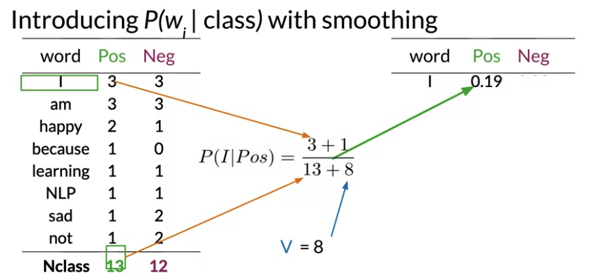
However, if a word does not appear in the training, then it automatically gets a probability of 0, to fix this we add smoothing as follows
\[P\left(w_i \mid positive \right) = \frac{freq\left(wi,positive \right) + 1}{N_{positive} + V}\] \[P\left(w_i \mid negative \right) = \frac{freq\left(wi,negative \right) + 1}{N_{negative} + V}\]where \(V\): the number of unique words in the entire set of documents(而不是total count of word), for all classes, whether positive or negative.
Log Likelihood
To compute the log likelihood, we need to get the ratios and use them to compute a score that will allow us to decide whether a tweet is positive or negative. The higher the ratio, the more positive the word is. To do inference, you can compute the following:
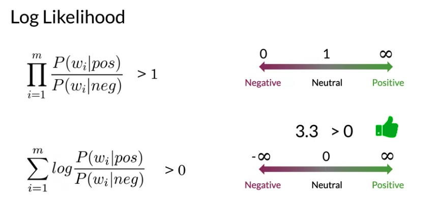
\[\frac{P\left(pos\right)}{P\left(neg\right)} \prod_{i=1}^m \frac{P\left(w_i \mid pos\right)}{P\left(w_i \mid neg\right)} > 1\]m gets larger, we can get numerical flow issues, hard to store on device , so we introduce the log, which gives you the following equation
\[log\left( \frac{P\left( D_{pos}\right)}{P\left(D_{neg}\right)} \prod_{i=1}^m \frac{P\left(w_i \mid pos\right)}{P\left(w_i \mid neg\right)} \right) => \underbrace{log\frac{P\left(D_{pos}\right)}{P\left(D_{neg}\right)}}_{\text{log prior}} + \underbrace{\sum_{i=1}^m log \frac{P\left(w_i \mid pos\right)}{P\left(w_i \mid neg\right)}}_{\text{log likelihood}}\] \[\text{where} \quad P\left(D_{pos}\right) = \frac{D_{pos}}{D}, P\left(D_{neg}\right) = \frac{D_{neg}}{D}\]- Reason to use log prior ratio: in real world, number of positive tweets may not equal to the number of negative tweets in your training data
- D is the total number of tweets
- \(D_{pos}\) is the total number of positive tweets and \(D_{neg}\) is the total number of negative tweets.
- 注:与\(N_{pos}\) 不同, \(N_{pos}\) 是total number of all positive words
log prior represents the underlying probability in the target population that a tweet is positive versus negative. important for unbalanced dataset. We further introduce λ as follows:
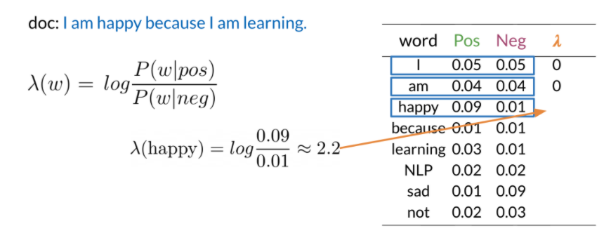
The positive value indicates tweet is positive. Negative value indicates tweet is negative
Training Naive Bayes
- collect and annotate corpus: divide tweets into two groups, positive/negative
- Preprocess the tweets: process_tweet(tweet) ➞ [w1, w2, w3, …]:
- Lowercase
- Remove punctuation, urls, names
- Remove stop words: Stop words are words that don’t add significant meaning to the text.
- Stemming
- Tokenize sentences
- Compute freq(w, class), use below table to compute
- Get \(P\left(w \mid pos \right), P\left(w \mid neg \right)\) using Laplacian Smoothing formula
- Get \(\lambda\left( w \right) = log \frac{P\left( w \mid pos \right)}{P\left( w \mid neg \right)}\)
- Compute \(logprior = log \frac{D_{pos}}{D_{neg}}\) where \(D_{pos}\) and \(D_{neg}\) correspond to the number of positive and negative documents respectively
Testing Naive Bayes
if a word not in vocabulary, think as neutral, not contribute to score
Naive Bayes Application
There are many applications of naive Bayes including:
- Author identification: document written by which author, calculate \(\lambda\) for each word for both author to build vocabulary
- Spam filtering: \(\frac{P\left(spam \mid email \right)}{P\left(nnspam \mid email \right)}\)
- Information retrieval: filter relevant and irrelevant documents in a database, calculate the likelihood of the documents given the query, retrieve document if \(\left( P\left(document_k \mid query \right) \approx \prod_{i=0}^{\mid query \mid} P\left(query_i \mid document_k \right) \right) > threshold\)
- Word disambiguation: e.g. don’t know bank in reading, refer to river or money? to calculate the score of the document, \(\frac{P\left(river \mid text\right)}{P\left(money \mid text\right)}\). if refer to river not money, score is bigger than 1.
Naive Bayes Assumption
Advantage: simple doesn’t require setting any custom parameters.
Assumption:
- Indepdence between predictors or features associated with each class
- assume word in a piece of text are independent. e.g. “It is sunny and hot in the Sahara desert.” But “sunny” and “hot” often appear together. And together often related to beach or desert. Not always independent
- Under or over estimate conditional probabilities of individual words e.g. “It’s always cold and snowy in ___” naive model will assign equal weight to the words “spring, summer, fall, winter”.
- Relative frequencies in corpus: rely on distribution on training dataset
- A good dataset contain the same proportion of positive and negative weets as a random sample. But in reality positive tweet is more common(because negative tweets maybe muted or banned by twitter). This would result a very optimistic or pessimistic model
Error Analysis
- Semantic meaning lost in the pre-processing step by removing punctuation and stop words (因为Naive Bayes removed Punctuation)
- “My beloved grandmother :(“, with punctuation indicating a sad face, after process, [belov, grandmoth], positive tweet
- “This is not good, because your attitude is not even close to being nice.” if remove neutral word, [good, attitude, close, nice] positive
- Word order affect meaning
- “I am happy because I did not go.” vs. “I am not happy because I did go.”
- Adversarial attack: some quirks of languages come naturally to human but confuse Naive Bayes model
- some common language phenomenon, Sarcasm, Irony and Euphemisms.
- e.g. “This is a ridiculously powerful movie. The plot was gripping and I cried right through until the ending” positive. After process. [ridicul, power, movi, plot, grip, cry, end] negative
1.3 Vector Space
e.g. “Where are you heading” vs “Where are you from” -> Different meaning 尽管前三个词一样
e.g. “What is your age” vs “How old are you” -> Same meaning
e.g. “You eat ceral from a bowl” ceral and bowl are related
e.g. “You can buy something and someone else sells it” second half sentence is dependent on the first half
- Vector space: identify the context around each word to capture relative meaning, to represent words and documents as vector
- Vector space allow to identify sentence are similar even if they do not share the same words
- Vector space allow to capture dependencies between words
- application:
- information extraction to answer questions in the style of who, what, where, how…
- machine translation
- chatbots programming: 机器客服
Word by Word Design
number of times they occur together within a certain distance k
Co-occurence matrix: e.g. data =2, count how many appearance for each word has distance smaller or euqal than 2
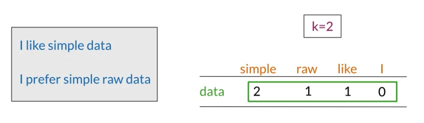
Word by word , get n entries, with n between 1 and size(vocabulary)
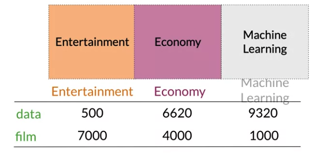
Word by Document Design
number of times they occur together within a certain category k
Divide corpus into different tops like Entertainment, Economy, Machine Learning. Below data appear 500 times in corpus related to Entertainment, 6620 times in documents related to Economy
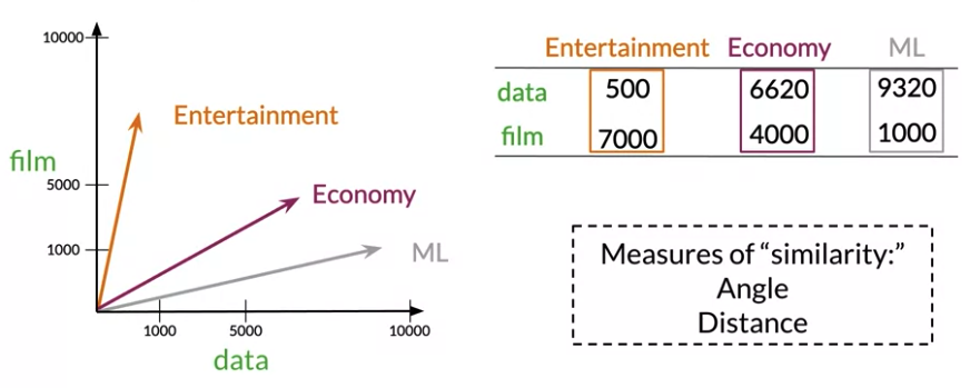
Euclidean Distance
Euclidean Distance is the norm of the difference between vectors, straight line between points
\[d\left( \vec{v}, \vec{w} \right) = \sqrt{\sum_{i=1}^n \left(v_i - w_i \right)^2 } \quad \rightarrow \quad \text{Norm of } \left( \vec{v}, \vec{w} \right)\]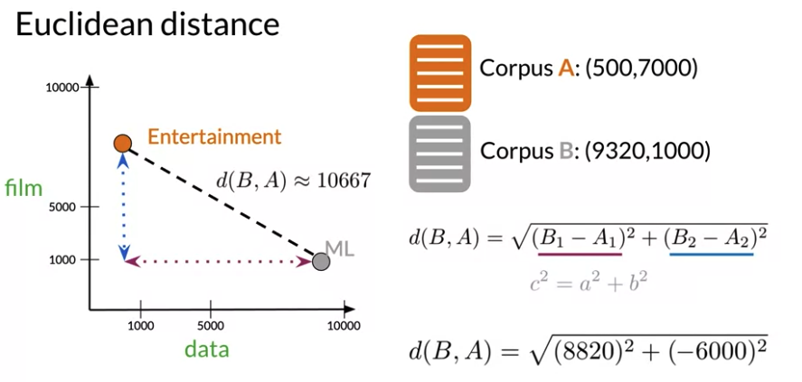
v = np.array([1,6,8])
w = np.array([0,4,6])

#Calculate the Eudlidean distance d

d = np.linalg.norm(v-w)
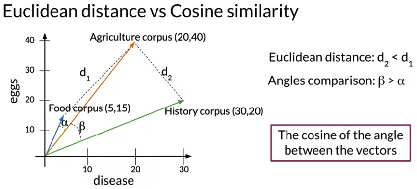
Cosine Similarity
Problem with Euclidean distance: Biased by the size of appearance. Vector space where corpora are represented by occurrence of the words “disease” and “eggs”. Because Agriculture and history corpus has a similar number of words(出现单词数量一样), Suggests agriculture and history 比 agriculture and food 更想近义
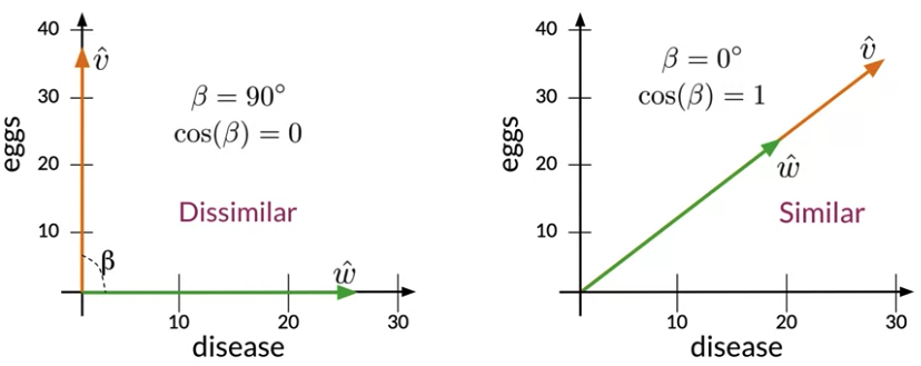
- if A and B are identical, you will get \(cos\left( \theta \right)=1\)
- If you get \(cos\left( \theta \right)=0\), that means that they are orthogonal (or perpendicular).
- Numbers between 0 and 1 indicate a similarity score.
- Numbers between -1 and 0 indicate a dissimilarity score.
- Advantage: Cosine similarity isn’t biased by the size difference between the representations
- proportional to the similarity between the directions of the vectors that you are comparing.
- the cosine similarity values between 0 and 1 for word by Word/Docs, cosine similarity values between -1 and 1 when using word embedding
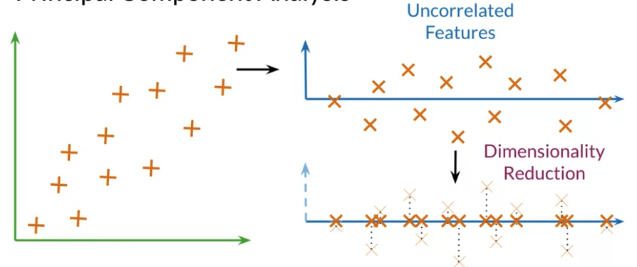
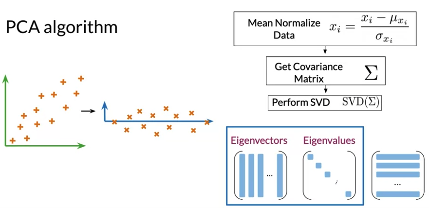
PCA
- PCA: dimenison reduction from high dimension to fewer dimension. project data into a lower dimension while retaining as much information as possible
- Original Space -> Uncorrelated features -> Dimension Reduction
- Can use visualization to check if PCA capure relationship among words
- Eigenvector: directions of uncorrelated features for your data
- Eigenvalue: amount of information retained by each feature(variances of data in each of those new features)
- Dot Product(between x and eigenvector): gives the projection on uncorrelated features
- Mean Normalize Data \(x_i = \frac{x_i - \mu_i}{\sigma_{x_{i}}}\)
- Get Covariance Matrix
- Perform Singular Value Decomposition to get set of three matrices(Eigenvectors on column wise, Eigenvalues on diagonal). Eigenvalues and eigenvectors should be organized according to the eigenvalues in descending order. Ensure to retain as much as information as possible
- Project data to a new set of features, using the eigenvectors and eigenvalues in this steps

1.4 Transforming word vectors
Translate word: calculate word embedding in English and French, transform word embedding in English to French and find the most similar one
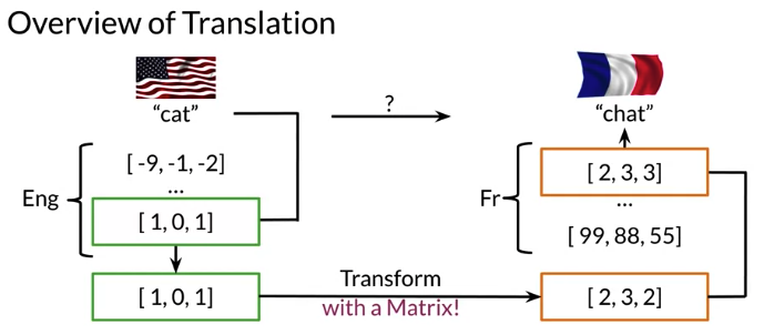
R: transform matrix, X: English word, Y: French word. First get subsets of English word and French equivalence
Why not store all vocabulary?: just need a subset to collect to find transform matrix. If it works well, then model can translate words that are not in vocabulary
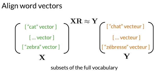
Solving for R:
\[\begin{align} \color{olive}{\text{Initialize R}}\quad & \\ \color{blue}{\text{in a loop:}}\quad & \\ & Loss = \Vert XR - Y \Vert_F \qquad \color{fuchsia}{\text{Frobenium Norm}} \\ & g = \frac{d}{dR} Loss \qquad \color{fuchsia}{\text{gradient R}} \\ & R = R - \alpha g \qquad \quad \color{fuchsia}{\text{update}} \end{align}\]Can pick a fixed number of times to go through the loop or check the loss at each iteration and break out loop when loss falls between a certain threshold.
Explanation for fixed number of iterations iterating until the loss falls below a threshold instead checking loss at each iteration.
- You cannot rely on training loss getting low – what you really want is the validation loss to go down, or validation accuracy to go up. And indeed - in some cases people train until validation accuracy reaches a threshold, or – commonly known as “early stopping” – until the validation accuracy starts to go down, which is a sign of over-fitting.
- Why not always do “early stopping”? Well, mostly because well-regularized models on larger data-sets never stop improving. Especially in NLP, you can often continue training for months and the model will continue getting slightly and slightly better. This is also the reason why it’s hard to just stop at a threshold – unless there’s an external customer setting the threshold, why stop, where do you put the threshold?
- Stopping after a certain number of steps has the advantage that you know how long your training will take - so you can keep some sanity and not train for months. You can then try to get the best performance within this time budget. Another advantage is that you can fix your learning rate schedule – e.g., lower the learning rate at 10% before finish, and then again more at 1% before finishing. Such learning rate schedules help a lot, but are harder to do if you don’t know how long you’re training.
Frobenius norm
\[\Vert A \Vert_F = \sqrt{\sum_{i=1}^m \sum_{j=1}^n \vert a_{ij}\vert^2 }\]e.g. has two word embedding and dimension is two, the matrix is 2x2
\[A = \begin{pmatrix} 2 & 2\\ 2 & 2\\ \end{pmatrix}\] \[\Vert A \Vert_F = \sqrt{2^2 + 2^2 + 2^2 + 2^2} = 4\]A = np.array([[2,2,],
[2,2,]])
A_squared = np.square(A)
print(A_squared) # array([[4,4,],
# [4,4,]])
A_Frobenious = np.sqrt(np.sum(A_squared))
Frobenius norm squared
\[\frac{1}{m} \Vert XR - Y \Vert_F^2\]- When we take the square of all non-negative (positive or zero) numbers, the order of the data is preserved. For example, if 3 > 2, 3^2 > 2^2
- Using the norm or squared norm in gradient descent results in the same location of the minimum.
- Squaring cancels the square root in the Frobenius norm formula. if no square and only square root, we would have to do more calculations
- divide by m: We’re interested in transforming English embedding into the French. Thus, it is more important to measure average loss per embedding than the loss for the entire dictionary (which increases as the number of words in the dictionary increases).
so the gradient will be:
Gradient
Easier to take derivative rather than dealing with the square root in Frobenius norm
\[Loss = \Vert XR - Y \Vert_F^2\] \[g = \frac{d}{dR}Loss = \frac{2}{m} X^T \left( XR - Y \right)\]Locality Sensitive Hashing
Reduce computational cost(much faster) to find K-nearest neighbor is to use locality sensitive hashing. For example, 蓝色点在蓝色plane 上方,灰色点在灰色plane上方
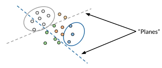
For text embedded vector, nearest neighbors refer to text with similar meaning, so can group certain vetors when find synonym by hashing => speed up searching
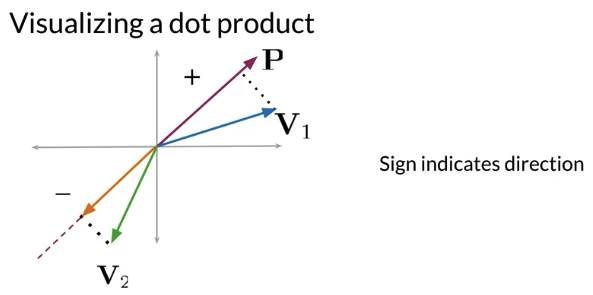
- If dot product positive, it’s on one side of the plane.
- If dot product negative, it’s on opposite side of the plane.
- If dot product is zero, it is on plane
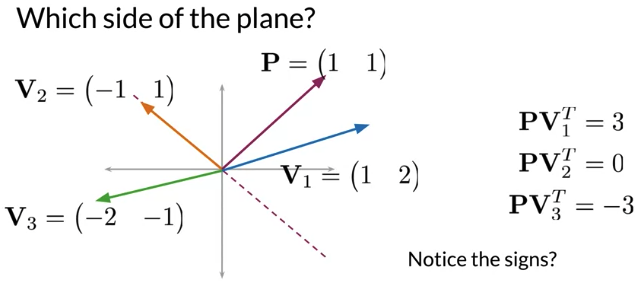
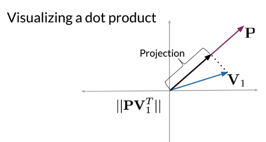
E.g. dot product of P and V1 is equal to the do length of P multiply V1 projection onto P
def side_of_plane(P,v):
  dotprodcut = np.dot(P,v.T)
  sign_of_dot_product = np.sign(dotproduct)
  sign_of_dot_prodcut_scalar = np.asscalar(sign_of_dot_product)
  return sign_of_dot_prodcut_scalar
Multiple Plane
To divide vector space into manageable regions, want to use more than one plane with a single hash value
\[\color{maroon}{\text{sign_i} \geq 0, \rightarrow h_i = 1}\] \[\color{maroon}{\text{sign_i} < 0, \rightarrow h_i = 0 }\] \[\mathbf{hash = \sum_i^H 2^i \times h_i}\]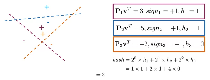
def hash_multiple_plane(P_l, v):
    hash_value = 0
    for i, P in enumerate(P_l):
        sign = side_of_plane(P,v)
        hash_i = 1 if sign >=0 else 0
        hash_value += 2**i * hash_i
    return hash_value
#Generate Random Plane

num_dimensions = 2
num_planes = 3

random_planes_matrix = np.random.normal(
                       size = (num_planes,
                               num_dimensions))
#[[ 1.76405235  0.40015721]

# [ 0.97873798  2.2408932 ]

# [ 1.86755799 -0.97727788]]

#find out whether vector v is on positive or negative side of each planes

def side_of_plane_matrix(P,v):
  dotproduct = np.dot(P,v.T)
  sign_of_dot_product = np.sign(dotproduct)
  return sign_of_dot_product

v = np.array([[2,2]])
num_planes_matrix = side_of_plane_matrix(random_planes_matrix, v)
#array([[1.],

#       [1.],

#       [1.]])

hashvalue = hash_multiple_plane(random_planes_matrix, v)
print(hashvalue) # 7
Application: find synonym for English word.
- Use word embedding transform word to embedding vector
1 x N_DIMS - Hash every word from vocabulary from above methods by calculate dot product between embedding vector and plane(
np.random.normal(size=(N_DIMS, N_PLANES))) - Find the synonym of word like “Apple” only from subset of vocabulary which has the same hash value of “Apple” (
hash_multiple_plane(P_l, Apple embedding vector))
2.1 Autocorrect and Minimum Edit Distance
How it works?
- Identify a misspelled word(only spelling error, not contextual error(e.g. Happy birthday to deer friend)) - how ? if spelled correctly, it is in dictionary. if not, probably a misspelled word
- Find strings n edit distance way e.g. deah vs dear
- Edit: an operation perfomed on a string to change it, including: insert, delete, switch (eta - > eat, eta -> tea, but not eta -> ate), replace
- Autocorrect: n is usually 1 to 3 edits
- Filter candidates
- step 2 generate word if not in vocabulary, remove it. e.g. deah -> d_ar, if d_ar not in vocabulary remove it
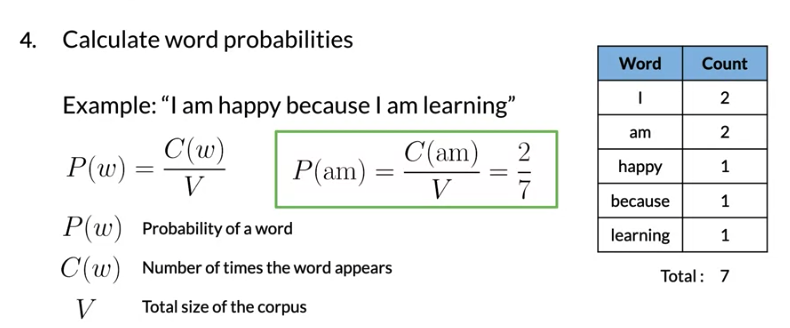
- Calculate word probabilities: \(P\left( w \right) = \frac{C\left( w \right) }{V}\), \(C\left( w \right)\)在文本中出现次数, V: total size of the corpus
Minimum distance application: spelling correction, document similarity, machine translation, DNA sequencing etc
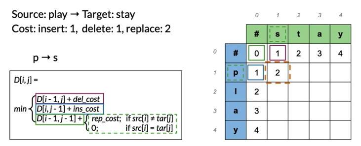
Minimum edit distance(Levenshtein distance): insert(cost 1), delete(cost 1), replace(cost 2, can think of delete then insert)
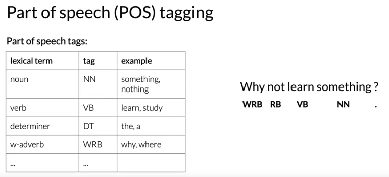
2.2 Part of Speech Tagging and Hidden Markov Models
Application:
- indentify entity: “Effel Tower is in Paris” Effel Tower & Paris are entities
- Co-reference resolution: “Effel Tower is in Paris, it is 324 meters high”, speech tagging indentify it refer to Eiffel Tower
- Speech Recognition: check if a sequence of word has a high probability or not
Markov chain
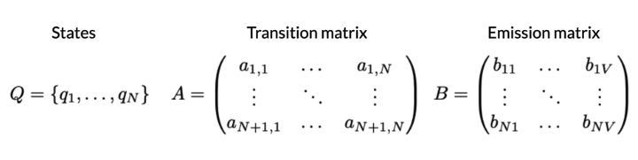
Markov chain: type of stochastic model that describes a sequence of possible events. To get probability of each event, it needs only the states of the previous events. Stochastic means random or randomness. Markov chain can be depicted as directed graph. A state refers to a certain condition of the present moment.
e.g. Why not learn … (next is verb? or norm?) depends on previous word
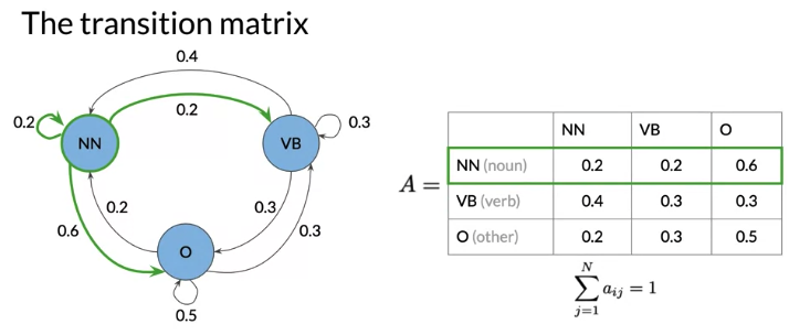
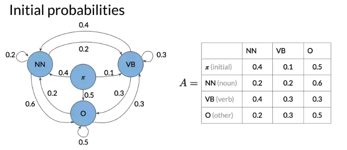
To predict the first word, because state depend on previous state, introduce initial state. Transition Matrix A (n+1) x n where n is the number of hidden states.
Hidden Markov Model
Emission probability: the transition from hidden states of Hidden Markov model(Noun, Verb…) to the words of corpus(I, am …). 从单词的词性 到 具体的单词的概率)
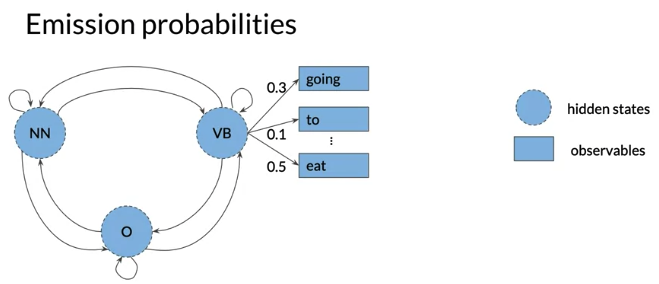
e.g. VB -> eat 0.5 means: 表示current hidden state is a verb, 0.5 chance that the model will emit the word eats. 注意 一样的的单词 不同的词性 , Emission probability 不同, 例如 He lay on his back V.S. I’ll be back
Calculate Probability
Process Corpus:
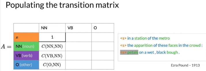
- Add start token in each line of sentence as to calculate initial probability
- transform all words in lowercase and keep punctuation
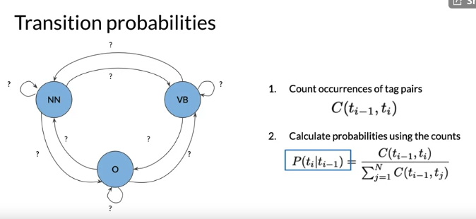
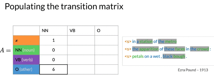
Calculate Transition Matrix:
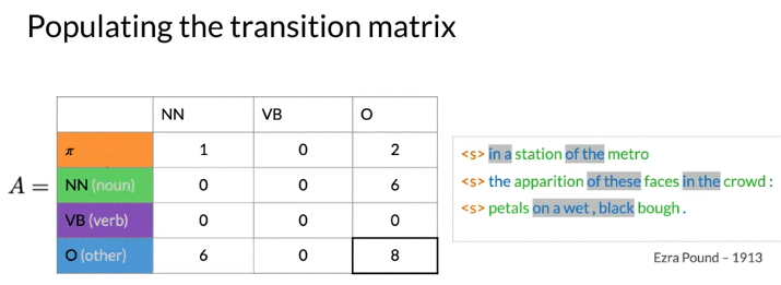
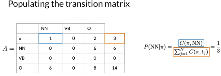
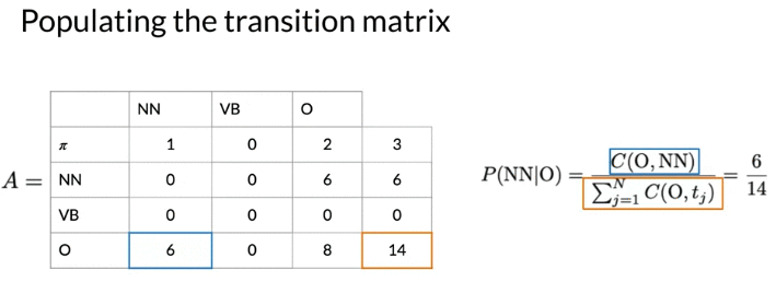
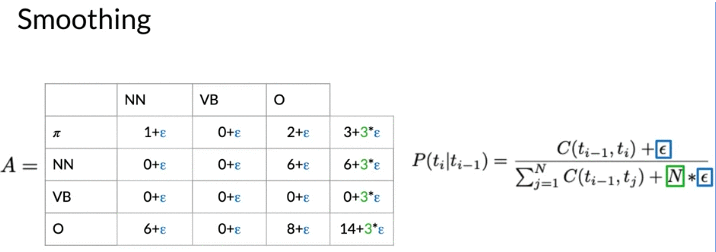
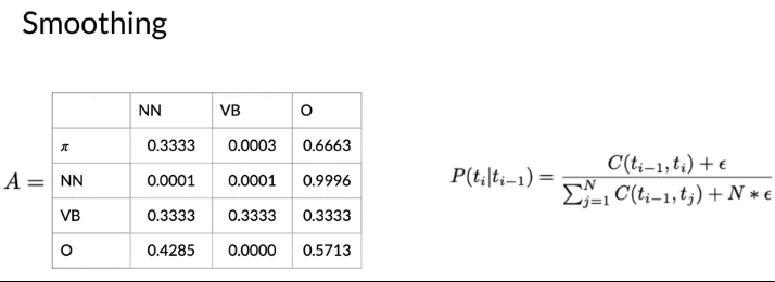
Soothing
- 为了避免probability as 0, add a small value eplison(e.g. 0.001)
- vb is 1/3 for all outgoing transitions. 是Reasonable的 because don’t have any data to estimate these probabilities
- In reall world, don’t apply smoothing for initial probability. Because: if add, allow a sentence to start with any parts of speech tag, including punctuation
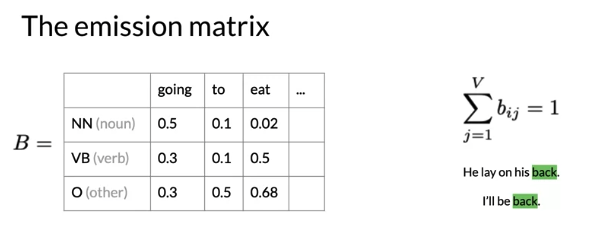
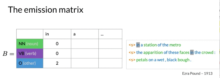
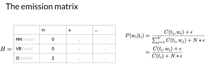
Populating the Emission Matrix
\(C\left(t_i \right)\): tag i 总共出现的次数,
\(C\left(t_i, w_i \right)\) word_i 属于tag_i 出现的次数
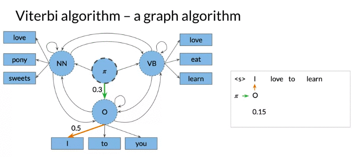
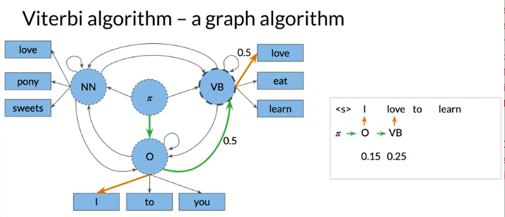
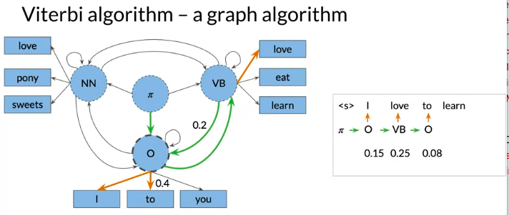
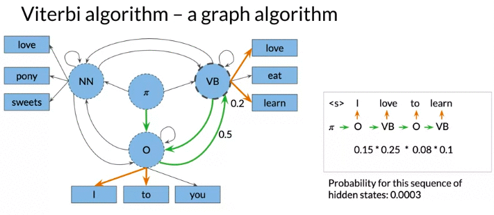
Viterbi Algorithm: a graph algorithm
To predict part-of-speech tags(辨认每个词的词性), can divide to two steps
- Predict Tag -> Tag (e.g. Noun -> Verb?) (Transition Probability)
- Predict Tag -> Word (e.g. Noun -> Math?) (Emission Probability)
下面例子: 注 from O -> NN 和 O - VB has the same probability. But the emission probability of love is higher for VB.
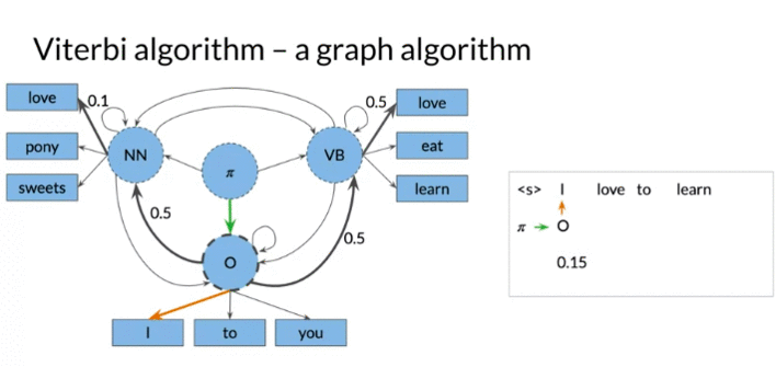
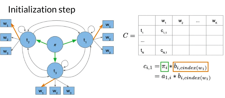
Viterbi Algorithm 通过两个matrix (C&D) 实现
- Matrix C: C(i,j) Given ith-tag word and j-th word, it hold the maximum probability so far.
- first column C: the product of transition probability of initial state (from initial state \(\pi\) to tag i) and emission probability. \(c_{i,1} = \pi_i \times b_{i,cindex\left(w_1\right)}\)
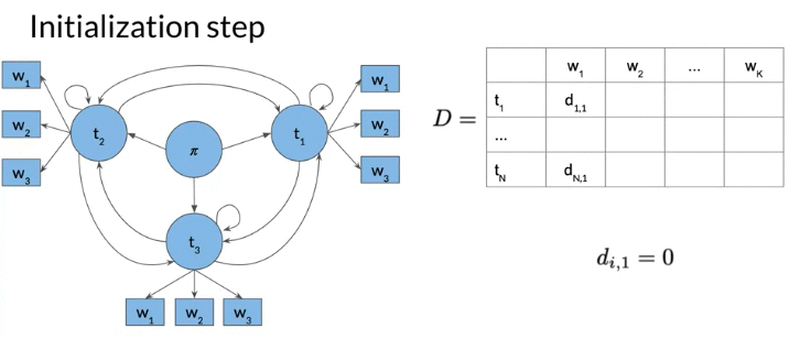
- Matrix D: D(i,j) Given i-th tag and j-th word, the optimal previous visited state index given word \(w_i\)
- The column 0 is all 0, no proceeding tags traversed
- Both matrix n rows: the number of speech tags/hidden states. K columns: the number of words in given sequences
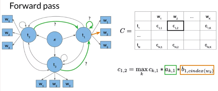
Forward Pass
Matrix C: \(c_{i,j}\): 第i个tag, 第j个单词
\[c_{i,j} = \underset{k}{max} \ c_{k,j-1} \times a_{k,i} \times b_{i,cindex\left(w_j\right)} \text{}\]- \(b_{i,cindex\left(w_j\right)}\): emission proability from \(tag_i\) to \(word_j\)
- \(a_{k,i}\) the transition probability from previous \(tag_k\) to current \(tag_i\)
- \(c_{k,j-1}\): the probability of proceeding path traversed 到 tag k, 第j-1 个text最佳的概率
- Then choose k to maximize the entire formula
In real word use log probability: to avoid multiply very small number, may lead to numeric issue for multiplication
\[c_{i,j} = \underset{k}{max} log\left(\ c_{k,j-1}\right) + log\left(a_{k,i}\right) + log\left(b_{i,cindex\left(w_j\right)}\right) \text{}\]Matrix D
\[d_{i,j} = \underset{k}{argmax} \ c_{k,j-1} \times a_{k,i} \times b_{i,cindex\left(w_j\right)} \text{}\]- in each \(d_{i,j}\) save the k which maximize the entry in \(c_{i,j}\)
- argmax returns k which maximize the function arguments instead of maximum value
In the below example, three states are not initial state, state can be 1,2,3. k can be 1,2,3
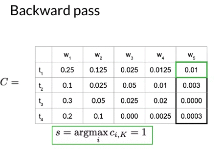
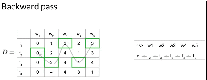
Backward Pass
Extract the graph from matrix D step by step
- Get the index of entry of \(C_{i,k}\) which is the highest probability in the last column C.
- Use that index s (\(\underset{i}{argmax} \ c_{i,k}\)) to traverse backwards through the matrix D to reconstruct the sequence. 从后往前推
e.g. 下面的例子,
- 最后一列的最大的概率是 \(C_{1,5} = 0.01\), \(s = \underset{i}{argmax} \ c_{i,k} = 1\). The most likely tag for 5th-word is tag1
- \(D_{1,5} = 3\), so previous index is 3 ( tag 3 is the pervious state with the highest proabability for \(C_{1,5}\))
- Algorithm stops as arrived at the start token
2.3 Autocomplete and Language Models
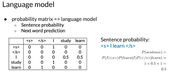
Language model: calculate the probability of a given sentence
- Estimate probability of word sequences.
- Estimate probability of a word following a sequence of words with most likely suggestions(Autocomplete a sentence) e.g. if you type, how are, e-mail application guess you
- It estimate the probability by splitting sentence into series of n-grams then find their probability in the probability matrix. Then language model predict next elements of sequence by return the word with highest probability
Application:
- Speech recognition: P(I saw a van) > P(eyes awe of an)
- Spelling correction
- Augmentatitve communication: predict most likely word from menu for people unable to physically talk or sign
- Augmentative communication system: take a series of hand gestures from a user to help them form words and sentences
N-gram
- An N-gram: sequence of N words. Order matters
- punctuation is treated as words. But all other special characters such as codes will be removed
E.g.
- Bigrams are all sets of two words that appear side by side in corpus. Notes: 下面例子,
I amappear twice, 但是only include 一次在 bigram set, I happy 因为不相邻,所以不是 bigram - Tigram: represent unique triplets of words that appear together in the sequence together in the corpus
Sequence Notation:
\[W_1^3: \text{sequence of words from word 1 to word 3}\] \[W_{m-2}^m: \text{sequence of wrods from word m-2 to word m}\]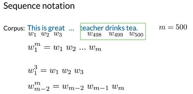
Probability
Note: in bigram: \(P\left( happy \mid I \right) = 0\) 因为 I happy never appear in the corpus
\[\text{Probabiity of bigram} \quad P\left( y \mid x \right) = \frac{ C\left(x, y \right)}{\sum_w{C\left(x, w \right)}} = \frac{ C\left(x y \right)}{C\left(x \right)}\] \[\text{where }C_\left(x \right): \text{the count of all unigram x.} \quad \sum_w{C\left(x, w \right)}: \text{the count of all bigram starting with x}\]\(\sum_w{C\left(x, w \right)}\) bigram can be simpilied to \(C_\left(x \right)\) unigram: only works if x is followed by another word
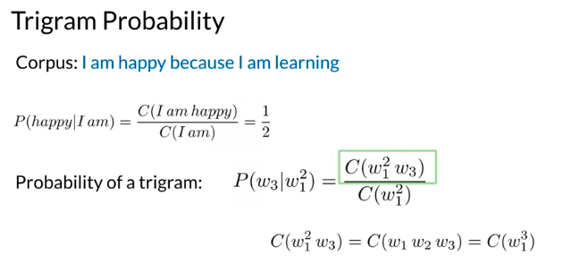
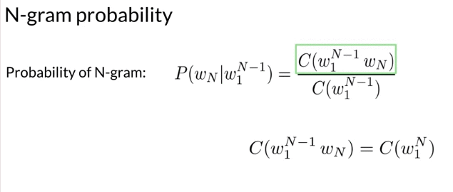
\[\text{Probabiity of trigram} \quad P\left( w_3 \mid w_1^2 \right) = \frac{ C\left(w_1^2 w_3\right)}{C\left(w_1^2\right)}\] \[C\left(w_1^2 w_3\right) = C\left(w_1 w_2 w_3 \right) \quad \text{a bigram followed by a unigram}\] \[\text{Probabiity of N-gram} \quad P\left( w_N \mid w_1^{N-1} \right) = \frac{ C\left(w_1^{N-1} w_N\right)}{C\left(w_1^{N-1}\right)}\]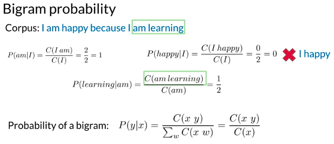
Problem with above calculation: Corpus almost never contains the exact sentences we’re interested in or even its longer subsequences, 比如\(C\left( the \ teacher \ drinks \ tea \right)\) and \(C\left( the \ teacher \ drinks \right)\) 可能都不会出现在 training corpus, the count are 0. 当sentences get longer and longer, the likelihood that more and more words will occur next to each other in the exact order gets smaller and smaller
Solution: use approximation: product of probabilities of bigrams
\[P\left(the \ teacher \ drinks \ tea\right) \approx P\left(the \right)P\left(teacher \mid the \right)P\left( drinks \mid teacher \right)P\left(tea\mid drinks \right)\]- Markov assumption: only last N words matter
- Bigram: \(P\left( w_n \mid w_1^{n-1} \right) \approx P\left( w_n \mid w_{n-1} \right)\)
- N-gram: \(P\left( w_n \mid w_1^{n-1} \right) \approx P\left( w_n \mid w_{n-N+1}^{n-1} \right)\)
- Entire sentence modeled with bigram: \(P\left( w_1^n \right) \approx \prod_{i=1}^{n} P\left( w_i \mid w_i-1 \right)\)
- contrast with Naive Bayes where approximate sentence probability without considering any word history (proability of i-th word condition on i-1 th word)
- \(P\left( w_1^n \right) \approx P\left(w_1 \right)P\left(w_2 \mid w_1 \right)P ... P\left(w_n\mid w_{n-1} \right)\): The first term of Bigram reiles on unigram probability of first word n sentence
Start & End of Sentences
Start:
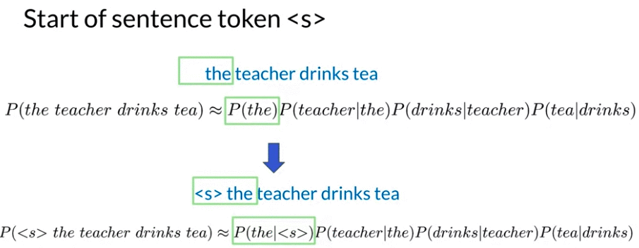
- Problem: first word, don’t have previous word, can’t calculate bigram probability for first word
- Solution: add a special term
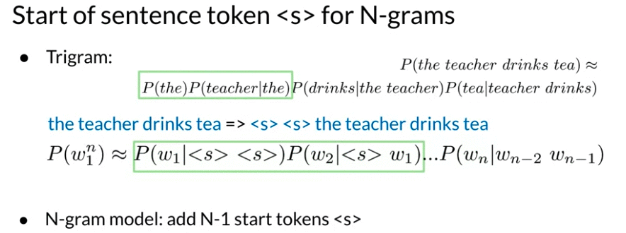
<s>so can calculate the probabilities - For n-grams, first N words, don’t have enough context, add n-1 special term
End:
Problem 1: \(\text{Probabiity of bigram} \quad P\left( y \mid x \right) = \frac{ C\left(x, y \right)}{\sum_w{C\left(x, w \right)}} = \frac{ C\left(x y \right)}{C\left(x \right)}\), \(\sum_w C\left(x, w \right)\) the count of all bigram starting with X. When x is last word of sentences, doesn’t work
e.g. Corpus:
<s> Lyn drinks chocolate<s> John drinks
Solution: add end of sentence token
Problem 2:
e.g. Corpus:
<s> yes no<s> yes yes<s> no no
all possible sentences of lengths 2: add all probability will equal to 1 👌
<s> yes yes, \(P\left( <{s}> yes \ yes \right) = \frac{1}{3}\)<s> yes no, \(P\left( <{s}> yes \ no \right) = \frac{1}{3}\)<s> no no\(P\left( <{s}> no \ no \right) = \frac{1}{3}\)<s> no yes\(P\left( <{s}> no \ yes \right) = 0\)
all possible sentences of lengths 3: add all probability will equal to 1 👌
<s> yes yes yes, \(P\left( <{s}> yes \ yes \right) = ...\)<s> yes no no, \(P\left( <{s}> yes \ no \right) = ...\)<s> no no no\(P\left( <{s}> no \ yes \right) = ...\)
However, What you want is the sum of all sentences of all length to 1: \(\sum_{2 word}P\left( ...\right) + \sum_{3 word}P\left( ...\right) ... = 1\)
Solution: add end of sentence token </s>
Bigram:
<s> Lyn drinks chocolate </s><s> John drinks </s>
e.g. Bigram:
<s> the teacher drinks tea => <s> the teacher drinks tea </s>
e.g. Bigram:
<s> Lyn drinks chocolate </s>\(P\left( sentence \right) = \frac{2}{3} * \frac{1}{2} * \frac{1}{2} * \frac{2}{2} = \frac{1}{6}\)<s> John drinks tea </s>\(P\left( sentence \right) = \frac{1}{3} * \frac{1}{1} * \frac{1}{2}* \frac{1}{1} = \frac{1}{6}\)<s> Lyn eats chocolate </s>\(P\left( sentence \right) = \frac{2}{3} * \frac{1}{2} * \frac{1}{1} * \frac{2}{2} = \frac{1}{3}\)
N-gram: => just one </s> at the end of sentences
e.g. Trigram:
<s> <s> the teacher drinks tea </s>
Count Matrix & Probability Matrix
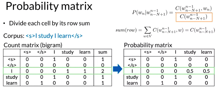
\[\text{Note: } P\left( w_n \mid w_{n-N+1}^{n-1} \right) = \frac{ C\left(w_{n-N+1}^{n-1}, w_n\right)}{C\left( w_{n-N+1}^{n-1}\right)}, w_n \text{ 表示第n个word}\]- Count Matrix row: unique corpus (N-1)-grams
- Count Matrix columns: unique corpus words
- Probability Matrix: divde each cell from Count Matrix by Count Matrix row sum
- Count Matrix row sum equivalent to your counts of n-1 gram: \(sum\left( row \right) = \sum_{w \in V} C\left(w_{n-N+1}^{n-1}, w\right) = C\left(w_{n-N+1}^{n-1}\right)\)
Log probability: all probability in calculation <= 1 and mutiplying them brings risk of underflow
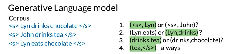
Algorithm
- Choose sentence start: randomly choose among all bigrams starting with
<s>based on bigram probability. Bigrams with higher probabilities are more likely to be chosen. - Choose next bigram starting with previous word from step 1 randomly, 概率更高,被抽到概率更大
- Continue until
</s>is picked
e.g. : choose 是绿色
Perplexity
\[\begin{align} Perplexity& = 2^{\text{entropy}} \\ & = 2^{-\sum_{i = 1}^N P \left( i \right) log_2 P\left( w_i \mid w_1, w_2, \cdots, w_{i-1} \right) }\\ &= e^{-\sum_{i = 1}^N P \left( i \right) ln p\left( w_i \mid w_1, w_2, \cdots, w_{i-1} \right) } \\ \text{Note: } ln P\left( w_i \mid w_1, w_2, \cdots, w_{i-1} \right) & \color{fuchsia}{\text{ is the prediction from log softmax}} \\ \text{Assume each word has} & \text{ the same probability/frequency for output} \\ &= e^{-\sum_{i = 1}^N \frac{1}{N} \left( i \right) ln P\left( w_i \mid w_1, w_2, \cdots, w_{i-1} \right) } \\ & = \prod_{i = 1}^N P\left( w_i \mid w_1, w_2, \cdots, w_{i-1} \right)^{-\frac{1}{N}} \\ & = \sqrt[N]{\prod_{i = 1}^N \frac{1}{P\left( w_i \mid w_1, w_2, \cdots, w_{i-1} \right)}} \end{align}\]Language Model Evaluation
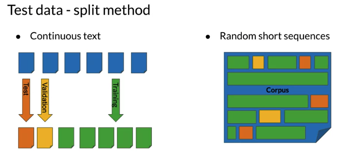
- For smaller corpora: 80% Train, 10% Validation(used for tuning hyper-parameters), 10% Test
- For large corpora(typical for text): 98% Train, 1% Validation(used for tuning hyper-parameters), 1% Test
- W : test set containing m sentence
- \(S_i\) i-th sentence in the test set, each ending with
</s> - N: number of all words in entire test set W including
</s>but not including<s> - Perplexity tells whether a set of sentences look like written by human or machine choosing words at random
- A text written by human => low perplexity score. Text generated by random word choice => high perplexity score
- Perplexity is the inverse probability of test sets normalized by the number of words in the test set => the higher the language model probability estimates => the lower perplexity will be
- Perplexity is closely related to entropy which measures uncertainty
- Good language model have perplexity score between 60 to 20. Log perplexity is between 4.3 and 5.9
- perplexity for character level language lower perplexity for than word-based model
- The same probability for different test sets, the bigger N the lower final perplexity will be
- Character level models Perplexity < word-based models Perplexity
e.g. 100 word in the text sets, N = 100, probability 0.9 which is high => means predict test sets very well
\[PP\left(W \right) = 0.9 => PP\left( W \right) = 0.9^{-\frac{1}{100}} = 1.00105416, \color{navy}{\text{very low perplexity}}\] \[PP\left(W \right) = 10^{-250} => PP\left( W \right) = \left(10^{-250} \right)^{-\frac{1}{100}} = 316, \color{navy}{\text{very high perplexity}}\]Perplexity for bigram model, m sentences and each sentences length is \(\mid s_i \mid\)
\[PP\left(W \right) = \sqrt[allword]{\prod_{i=1}^{m} \prod_{j=1}^{ \mid s_i \mid} \frac{1}{ P\left( w_j^{\left(i\right)} \mid w_{j-1}^{\left(i\right)} \right) }}, \,\, \color{red}{w_j^{\left(i\right)}\text{: j-th word in i-th sentence}}\]If all sentences in the test cases are concatenated:
\[PP\left(W \right) = \sqrt[N]{\prod_{i=1}^{N} \frac{1}{ P\left( w_i \mid w_{i-1} \right) }} = \sqrt[N]{\prod_{i=1}^{N} \frac{C\left( w_{i-1}, w_i \right)}{ C \left( w_{i-1}\right) }} \,\, \color{red}{w_i \text{: i-th word in test set}}\]Use log perplexity insetad of perplexity
\[logPP\left(W \right) = -\frac{1}{N}\sum_{i=1}^{N} log_2\left(P\left( w_i \mid w_{i-1} \right) \right), \,\, \color{red}{w_i \text{: i-th word in test set}}\]for i in range(sentence):
bigram = tuple(sentence[i: i + 2])
probability = probability * bigram_probabilities[bigram]
M = len(sentence)
perplexity = probability ** (-1 / M)
For Language model output activation LogSoftmax, model output i-th word is conditional log probability \(P\left( w_i \mid w_1, w_2 \cdots, w_{i-1} \right)\)
For a sentence containing N words
\[\begin{align} \text{log perplexity} & = log \left( \prod_{i=1}^N \frac{1}{P\left( w_i \mid w_1, w_2 \cdots, w_{i-1} \right)} \right)^{\frac{1}{N}} \\ & = - {\frac{1}{N}}\left( \sum_{i=1}^N log P\left( w_i \mid w_1, w_2 \cdots, w_{i-1} \right) \right) \end{align}\]For output pred dimension is (batch_size, #timestamp, Vocab Size ) and target(labe) dimension is (batch_size, #timestamp)
#**********************  Method 1 *************************

total_log_ppx = np.sum(preds*tl.one_hot(target, preds.shape[-1]) , axis= -1) # HINT: tl.one_hot() should replace one of the Nones,

non_pad = 1.0 - np.equal(target,  vocab['<PAD>'])
ppx = total_log_ppx * non_pad # Get rid of the padding, (batch_size, timeStamp)

log_ppx = np.sum(ppx) / np.sum(non_pad)


#**********************  Method 2 *************************

outputs = np.argmax(pred,axis=-1)
mask = 1 - np.equal(labels, pad) # or labels != pad

log_ppx = np.sum((outputs==labels)*mask)/np.sum(mask)
Out of vocabulary
- closed vocabulary: a fixed last of word. a set of unique word supported by a language model. e.g. chatbot only answer limited questions
- open vocabulary: can deal with words not seen before (out of vocabulary)
- unknown word also called out of vocabuarly word (OOV)
- replace unknown word with special tag
<UNK>in corpus and in input
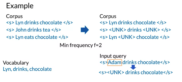
Using <UNK> in corpus
- create vocabulary V
- Criteria 1: min word frequency f: 至少在corpus 中出现f回
- Criteria 2: max size of vocabulary, only include words sort by frequency to the maximum vocabulary size
- Replace any word in corpus and not in V by
<UNK> - Count the probabilities with
<UNK>as with any other word,<UNK>usually lower perplexity
Note:
- You might have lot of
<UNK>, then model generate a sequence of<UNK>quotes with high probability instead of meaningful sentences. Due to this limitation, using<UNK>sparingly - Only compare Language model perplexity with the same vocabulary
比如下面例子,vocabulary 的词必须要在corpus中至少出现两回, 如果没有出现两回用 <UNK> 代替
Smoothing
Problem: N-gram made of known words still migh be missing in training corpus. 比如 eat chocolate. John drinks, bigram John eat are missing in bigram

Add-one smooething (Laplacian smoothing): add one occurence to each bigram. bigram that are missing in the corpus have nonzero probability. add one in each cell in the Count Matrix
\[P\left( w_n \mid w_{n-1} \right) = \frac{ C\left(w_{n-1}, w_n\right) + 1}{\sum_{w \in V} C\left( w_{n-1}, W\right) + 1} = \frac{C\left(w_{n-1}, w_n\right) + 1}{C\left(w_{n-1}\right) + V}\]Note: V is the size of vocabulary (而不是total count of word)
Plus V only works if real counts are large enough to outweigh the plus one. Otherwise the probability of missing word will be too high,比如就vocubary size = 2, \(P\left(\text{unk} \mid \text{known word} \right) = \frac{C\left(w_{n-1}, w_n\right) + 1}{C\left(w_{n-1}\right) + V} = \frac{1}{1 + 2} = \frac{1}{3}\)
Add-k smooething: make probability even smoother. can be applied to high order n-gram probabilities like trigram, four grams and beyond
\[P\left( w_n \mid w_{n-1} \right) = \frac{ C\left(w_{n-1}, w_n\right) + k}{\sum_{w \in V} C\left( w_{n-1}, W\right) + k} = \frac{C\left(w_{n-1}, w_n\right) + k}{C\left(w_{n-1}\right) + k*V}\]some other advanced smoothing: Kneser-Ney smoothing, Good-Turing smoothing
e.g. Corpus “I am happy I am learning” and k = 3, vocabulary size is 4 (I, am), (am, happy), (happy, I), (am, learning), (I, am) count is 2
Backoff
- if N-gram missing => using (N-1) gram. if (N-1) gram missing, using (N-2) gram… so on until find nonzero probabilities
- using lower level N-gram, distort probabilities especially for smaller corpora
- Probability need to be discounted from high probability to lower probability e.g. Katz backoff
- a large web-scale corpus : “stupid” backoff: no probability discounting applied. If high order n-gram probability is missing, the lower order n-gram probability is used by multiplying a constant. 0.4 is the constant expertimentally shown to work well
Linear Interpolation
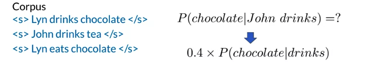
linear interpolation of all orders of n-gram: combined weighted probabilities of n-gram, (n-1) gram down to unigrams. Lambda are learned from validation parts of the corpus. Can get them by maximizing the probability of sentences from the validation set. The interpolation can be used for general n-gram by using more Lambdas
\[\hat P\left( w_n \mid w_{n-2}w_{n-1} \right) = \lambda_1 \times P\left( w_n \mid w_{n-2}w_{n-1} \right) +\lambda_2 \times P\left( w_n \mid w_{n-2} \right) + \lambda_3 \times P\left( w_n \right), given \sum_i \lambda_i = 1\]e.g. John drink chocolate
\[\hat P\left( chocolate \mid John \, drink \right) = 0.7 \times P\left( chocolate \mid John \, drink \right) +0.2 \times P\left( chocolate \mid drink \right) + 0.1 \times P\left( chocolate \right)\]2.4 Word Embeddings with Neural Networks
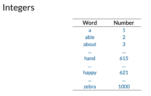
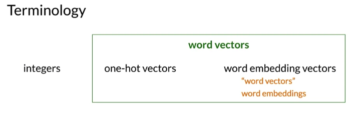
Build a vocabulary: assign integer to word, Problem: order doesn’t make sense from a semantic perspective. e.g. no reason that happy number > zebra
one-hot vectors
- put 1 in the row that has the same label and 0 everywhere else,
- Advantage: not imply any relationship between any two words. e.g. Each vector says the word either happy or not , either zebra or not
- Disadvantage:
- Huge vectors: require a lot of space and processing time. If created with English word, may have 1 million rows, one row for each English word
- No embedding meaning: if calculate the distance between one-hot vectors, always get the same distance btween any two pairs of words.
d(paper, excited) = d(paper, happy) = d(excited, happy), (inner product of any 2 one-hot vector is zero). 但是intuitively, happy is more similar to excited than paper
e.g. each vector has 1000 elements,
Word Embedding
比如横坐标,word are positive right, word are negative left; 纵坐标 word are concrete, higher. word are abstract lower. Less precise than one hot vector, 可能有两个点重合,比如snake & spider
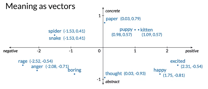
上面例子是一个word embedding.
- Low dimension: Word embedding represent words in a vector form that has a relative low dimension
- Carry embed meaning:
- e.g. semantic distance: \(\text{forst} \approx \text{tree, forest} \not\approx \text{ticket}\)
- e.g. analgies : Paris -> France similar as Rome -> Italy
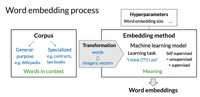
Create Word Embedding
- If you want to generate word embedding based on Shakespeare, corpus should be full and original text of Shakespeare, not study notes, slide presentation or keywords from Shakespeare.
- Context(combination of words to occur around that particular word) is important, give meaning to each word embedding. a simple vocabulary list of Shakespeare’s most common words not enough to create embedding.
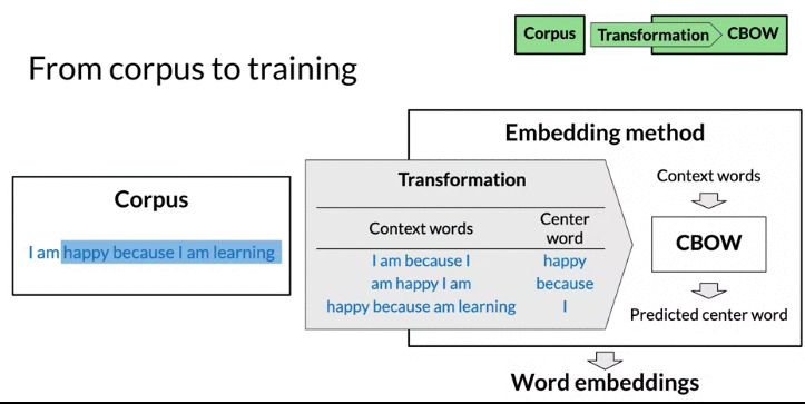
- Objective of word embedding: predict missing word given context words
- Embedding method, machine learning models which are set to learn word embeddings. The meaning of words, as carred by word embeddings depends on the embedding approach
- Self-supervised learning: Both unsupervised (input data are unlabeled) and supervised(text provide necessary context which would ordinarily make up the label)
- Word embedding can be tuned by a number of hyperparameters. 其中一个是 dimension of word embedding vectors. In practice, could from a few hundred to low thousand
- Use high dimension captures more nuanced meanings but computatitional expensive, may leading to diminishing return
- Corpus must first be transformed into a suitable mathematical representation. e.g. Integer word Indices or one-hot vector
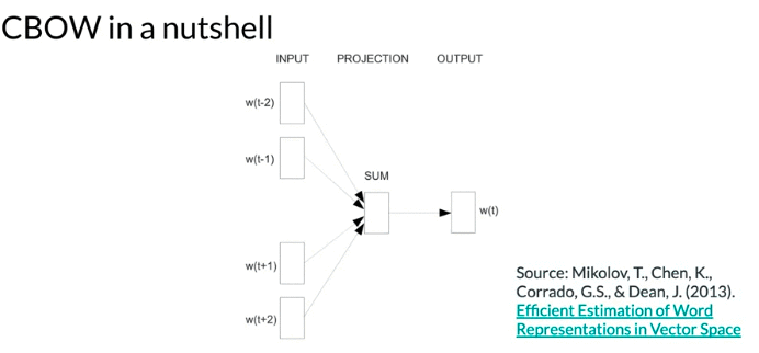
- word2vec: (Google, 2013). use a shallowed neural network to learn word embedding. propose two model architectures:
- Continuous bag-of-words(CBOW): predict a missing word given the surrounding words
- Continuous skip-gram also know as Skip-gram with negative sampling (SGNS): did the reverse of Continuous bag-of-words: model predict surrounding given a input word
- Global Vectors(GloVe) (Standford 2014): Involves factorizing the logarithm of the corpuses word co-occurrence matrix.(Similar to Count Matrix as above)
- fastText (Facebook 2016): based on skip-gram model and take into account the structure of words by representing words an n-gram of character
- support out-of-vocabulary(OOV) words: infer embedding from the sequence of characters they are made of and corresponding sequence that it was intially trained on. E.g. create similar embedding for kitty and kitten even kitty never seen before(因为 kitty and kitten has similar sequences of characters)
- another benefit: embedding vectors can be averaged together to make vector representations of phrases and sentences
- Advanced work embedding methods: use advanced deep neural network to refine word meanings according to their contexts. 一词多义(polysemy or words with similar meanings), 之前model always has the same embedding. In these advanced models, words can have different embeddings depending on their contexts. e.g. plants. 可以是 organism like a flower, a factory or adverb. below are Tunable pre-trained model available
- BERT (Google, 2018): Bidirectional representations from transformers by Google
- ELMo (Allen Institute for AI, 2018)P embeddings from language models
- GPT-2 (OpenAI,2018): generative pre-training 2
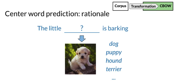
Continuous bag-of-words
- the objective: predict a missing word based on the surrounding words
- rationale: if two unique words are both frequently surrounded by a similar set of words in various sentences, then 这两个词 tend to related in their meaning(related semantically)
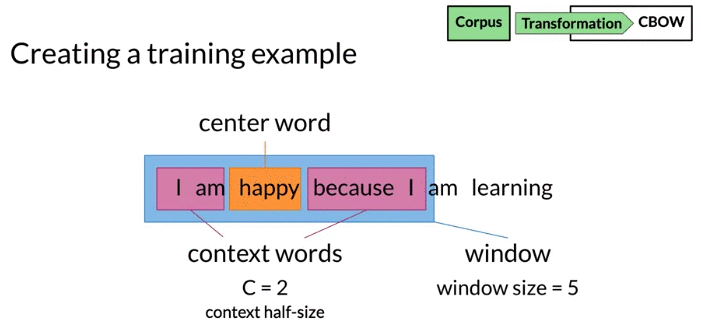
- define context words as four words. C= 2 Two words before center word and two words after it. C is half size of the context. C is the hyperparameter of the model
- Window: center word + context words
- Architecture: context words as input and center words as output
Tokenization
- Case insensitive: The==the==THE -> convert to either all lowercase or all uppercase
- Punctuation
- interruption punctuation marks
,!.?as single special word of the vocabulary. - ignore non interrupting punctuation marks
'<< >>" - collapse multi-sign marks into single marks
!!!->.,...->.
- interruption punctuation marks
- Number:
- If numbers do not carry important meaning -> drop
- number may have meaning. e.g. 3,1415926 -> pi, 90210 is name of television show and zip code => keep as
/<NUMBER>
- Special characters: such as mathematical symbols, currency symbols, section and paragraph signs and line markup signs => drop
- Special words: emojis, hastags (like twitter) => depend on if and how handle
- can consider each emoji or hashtag considered as individual word. 😄 ->
:happy
- can consider each emoji or hashtag considered as individual word. 😄 ->
# pip install nltk

#pip install moji

import nltk
from nltk.tokenize import word_tokenize
import emoji

nltk.download('punkt') #download pre-trained Punkt tokenizer for English

# handle common special uses of punctuation
下面例子, question marks and exclamation convert to a single full stop, last step get rid of number but keep alphabetical, full stops(previously an interrupting punctuation mark), emoji
corpus = 'Who ❤️ "word embeddings" in 2020? I do!!!'
import nltk
from nltk.tokenize import word_tokenize
import emoji

nltk.download('punkt')  # download pre-trained Punkt tokenizer for English

data = re.sub(r'[,!?;-]+', '.', corpus)
print(f'After cleaning punctuation:  {data}')
# After cleaning punctuation:  Who ❤️ "word embeddings" in 2020. I do.

data = nltk.word_tokenize(data)
print(f'After tokenization:  {data}')
# After tokenization:  ['Who', '❤️', '``', 'word', 'embeddings', "''", 'in', '2020', '.', 'I', 'do', '.']

data = [ ch.lower() for ch in data
         if ch.isalpha()
         or ch == '.'
         or emoji.get_emoji_regexp().search(ch)
       ]
print(f'After cleaning:  {data}')
# After cleaning:  ['who', '❤️', 'word', 'embeddings', 'in', '.', 'i', 'do', '.']
def get_windows(words, C):
    i = C
    while i < len(words) - C:
        center_word = words[i]
        context_words = words[(i - C):i] + words[(i+1):(i+C+1)]
        yield context_words, center_word
        i += 1
for x, y in get_windows(
            ['i', 'am', 'happy', 'because', 'i', 'am', 'learning'],
            2
        ):
    print(f'{x}\t{y}')
# ['i', 'am', 'because', 'i']	happy

# ['am', 'happy', 'i', 'am']	because

# ['happy', 'because', 'am', 'learning']	i
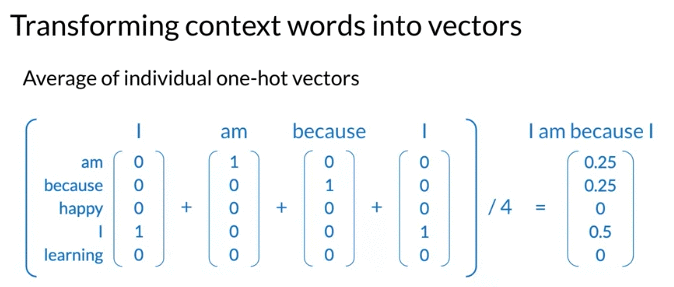
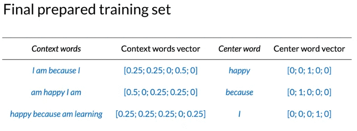
Transforming Words Into Vectors
Corpus: I am happy because I am learning
Vocabulary: am, because, happy, I, learning (vocabulary is the set of unique set)
- Center word: One-hot vector: 下面例子order by alphabetic order,实际中可以是arbitrary
- Context word: take the average of one-hot vectors of each context word (average 除以的是 2C, C is half size of context words )
def word_to_one_hot_vector(word, word2Ind, V):
  #word2Ind, word is key, index is value

    one_hot_vector = np.zeros(V)
    one_hot_vector[word2Ind[word]] = 1
    return one_hot_vector

context_words = ['i', 'am', 'because', 'i']
context_words_vectors = [word_to_one_hot_vector(w, word2Ind, V) for w in context_words]
# [array([0., 0., 0., 1., 0.]),

# array([1., 0., 0., 0., 0.]),

# array([0., 1., 0., 0., 0.]),

# array([0., 0., 0., 1., 0.])]

np.mean(context_words_vectors, axis=0)
# array([0.25, 0.25, 0.  , 0.5 , 0.  ])
Python- Create One hot vector for center /context word
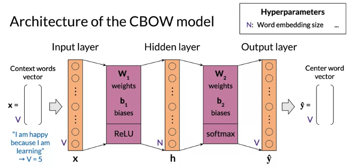
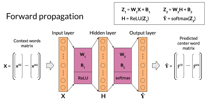
Architecture of Continuous bag-of-words
- based on shallow dense neural network with an input layer, a single hidden layer, and an output layer
- input is vector of context words, size(vector) = size(vocabulary) V
- output is predict of center word, size(vector) = size(vocabulary) V
- Hyparameter: word embedding size N = size (Hidden layer), typical from hundred to thousands
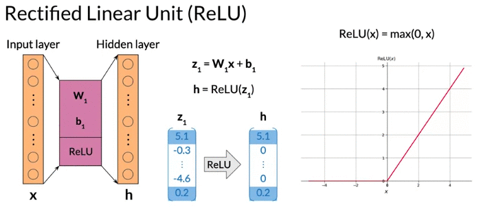
- Need activation function for hidden layer and output layer, result of activation layer is sent to next layer. The outcome of activation of output layer is model prediction
- Activation function: Hidden layer use ReLu, output layer use softmax
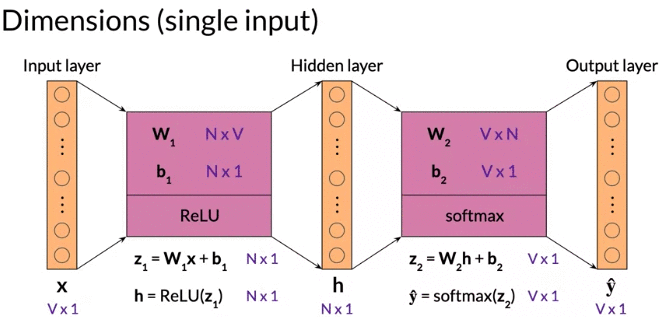
Dimension(single input): \(W_1\) : N (size of word embedding) rows and V (size of vocabulary ) columns

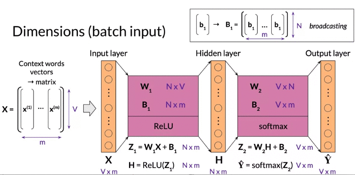
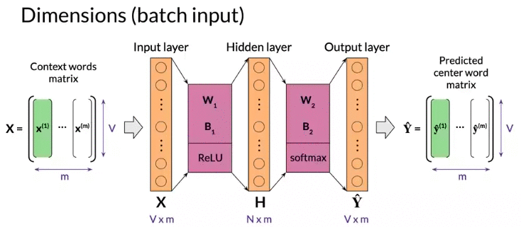
Dimension(Batch input): m: batch size: hyperparameter model defined at training time
note: \(b_1\) size is Nx1 broadcasting to NxM
Activation Function
Activation function: Hidden layer use ReLu, output layer use softmax
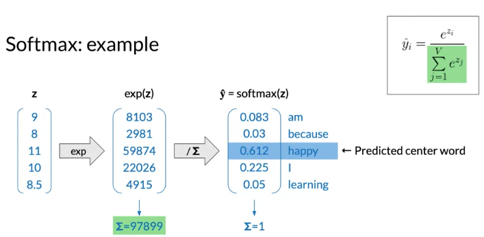
Softmax: input is a vector of real numbers. Output is a vector of real number in the interval 0 to 1 which sum up to 1, 可以被解释为 probabilities of exclusive events. Each row correspond to a word of the vocabulary: probability of being center word
\[\hat y_i = \frac{e^{z_i}}{\sum_{j=1}^{V}e^{z_j}}, \text{exponential form transform inputs to all positive }\]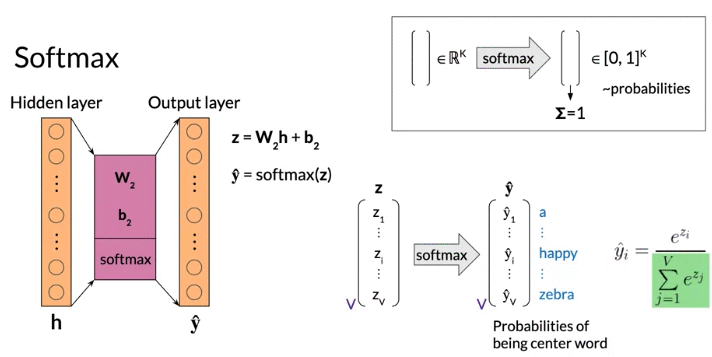
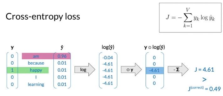
Cost Function
- find the parameters that minimize the loss given the training data sets
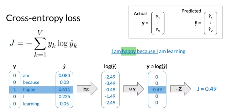
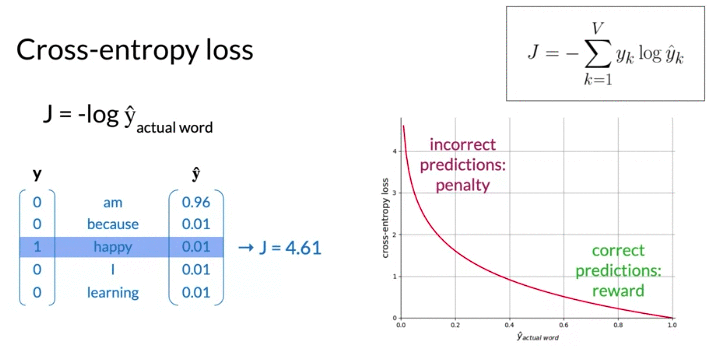
- loss function is cross-entropy loss(often used with classification models) -> used in logistic function (log loss)
- larger the loss when prediction incorret(见下面例子)
- when \(\hat y\) close to 1, cross entropy loss close to 0
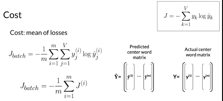
- loss refer to single example, cost refer to batch input(mean of losses)
Forward prop
Backward prop
- hyperparameter: learning rate \(\alpha\), alpha is small positive number less than 1.
Mathematical Prove:
Cost Function:
\[J = -\frac{1}{m} \sum_{i=1}^m y^{\left( i \right)} log a^{\left( i \right)}\]As we know:
\[d\frac{f\left(x\right)}{g\left(x\right)} = \frac{f'\left(x\right) g\left(x\right) - g'\left(x\right)f\left(x\right)}{g\left(x\right)^2}\]We define simplified notation
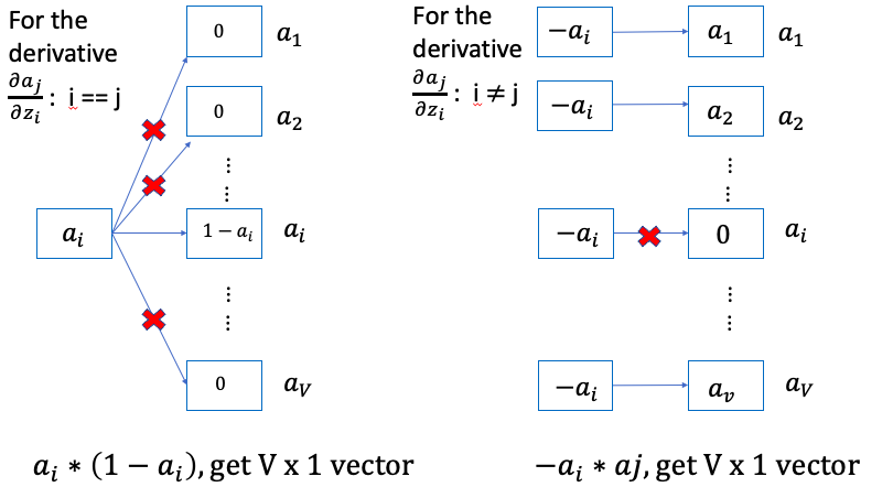
\[\text{Denote} \sum_i^V e^{z_i} \ = \sum, \text{ Denote } \hat a \left( \text {or } \hat y \right) \text{ is the activation output of softmax function}\]For \(i == j\):
\[\begin{align} \frac{\partial \frac{e^{z_i}}{\sum} }{\partial z_i} &= \frac{ e^{z_i} \sum - e^{z_i} e^{z_i} }{ \sum ^2} \\ &= \frac{e^{z_i}}{\sum} \frac{\sum - e^{z_i}}{\sum} = a_i \left( 1- a_i \right) \end{align}\]For \(i\neq j\):
\[\frac{\partial \frac{e^{z_i}}{\sum} }{\partial z_j} = \frac{ 0 \sum - e^{z_i} e^{z_j} }{ \sum ^2} = - a_i \, a_j\]So the derivative of softmax:
\[\frac{\partial a_i}{\partial z_j} = \begin{cases} a_i \times \left( 1- a_i \right) , & \text{if i = j} \\ - a_i \times a_j , & \text{if i } \neq \text{j} \end{cases}\] \[\text{Note: } y^{\left(i\right)}, \hat y^{\left(i\right)} \text{are label and predict(number) } i^{th} \text{word}\] \[\text{As we know }\sum_{i=1}^V a_i = 1\]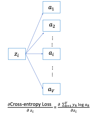
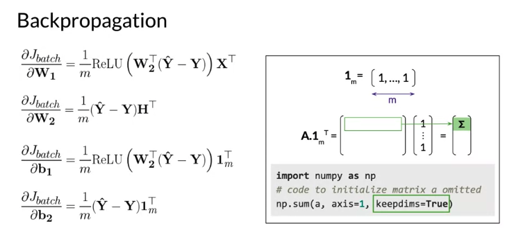
Vectorization Representation:
Therefore: Note \(a_1\) is the hidden layer output
\[\frac{\partial Cross-entropy \, Loss}{\partial W_2} = \frac{\partial Cross-entropy \, Loss}{\partial z} \frac{\partial z }{\partial w_2} = \frac{1}{m} \left( a -y \right) a_1^T\] \[\frac{\partial Cross-entropy \, Loss}{\partial b_2} = \frac{\partial Cross-entropy \, Loss}{\partial z} \frac{\partial z }{\partial b_2} = \frac{1}{m} \sum_{batch} \left( a -y \right)\] \[\frac{\partial Cross-entropy \, Loss}{\partial a_1} = \frac{\partial Cross-entropy \, Loss}{\partial z} \frac{\partial z }{\partial a_1} = W_2^T \left( a -y \right)\]The ReLu function derivative:
\[d Relu \left( x \right) = \begin{cases} 1 , & \text{if x > 0} \\ 0 , & \text{if x < 0 } \end{cases}\] \[\begin{align} \frac{\partial Cross-entropy \, Loss}{\partial W_1} & = \frac{\partial L }{\partial a_1} \frac{\partial a_1 }{\partial z_1} \frac{\partial z_1 }{\partial W_1} \\ & = \frac{1}{m} \left( W_2^T \left( a -y \right) \odot dZ \right) X^T \end{align}\] \[\begin{align} \frac{\partial Cross-entropy \, Loss}{\partial b_1} & = \frac{\partial L }{\partial a_1} \frac{\partial a_1 }{\partial z_1} \frac{\partial z_1 }{\partial b_1} \\ & = \frac{1}{m} \sum_{batch} \left( W_2^T \left( a -y \right) \odot dZ \right) \end{align}\]where \(\odot\) denote element-wise dot product and
\[dZ = \begin{cases} 1 , & \text{if } z = W_1 X + b > 0 \\ 0 , & \text{if } z = W_1 X + b < 0 \end{cases}\]Extract Word Embedding Vectors
After iterate training data serval times,
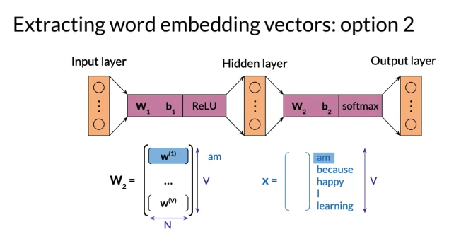
Option 1: can consider each column of \(W_1\) as embedding vector of a word of the vocabulary, \(W_1\) size is NxV, it has one column for each word in the vocabulary, 比如下面例子,总共5列,第一列 is the word embedding column vector for am, 第二列for because
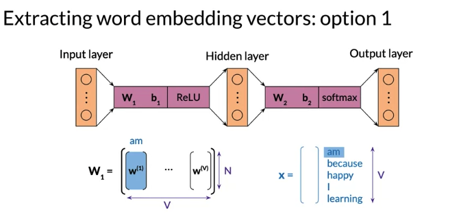
Option 2: Use each row in \(W_2\) as the embedding row vector for corresponding word. \(W_1\) size is VxV, order is the same as input vector or matrix 比如 第一行表示 embedding row vector for am, 第二行for because
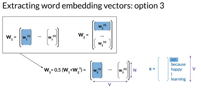
Option 3: average of Option 1 and Option 2, average \(W_1\) and the transpose of \(W_2\) , \(W_3\) size is NxV, each column of \(W_3\) as embedding vector of a word of the vocabulary, e.g. 第一列 is the word embedding column vector for am, 第二列for because
Evaluation
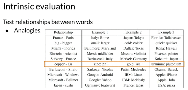
- Intrinsic evaluation: assess how well word embedding inherently capture the semantic(meaning of words) or syntactic(grammar) relationship between words
- could testing word embeddings on analogies:
- Semantic analogies: e.g. France -> pairs as Italy -> ?
- syntactic analogies: e.g. plural, tenses(时态), and comparatives(比较级) e.g. seen -> saw as been -> ?
- should aviod ambiguiy: may several correct answer e.g. wolf -> pack as bee -> swarm? colony?
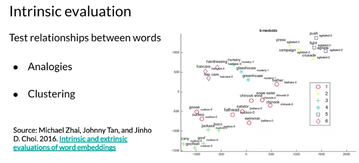
- Clustering: group similar word embedding vectors, capture related words. could be auomated using human made reference such as thesaurus(分类词汇汇编;百科全书)
- 比如下面例子 hair care & hairdressing close to each other
- could testing word embeddings on analogies:
- Extrinsic evaluation:use word embeddings to perform an external task, typically real world task that initially needed the word embeddings for. Then use performance metric of this task as a proxy for the quality of word embeddings
- task include: named entity recognition, parts-of-speech tagging
- A named entity can be referred to a proper name. e.g. “Andrew works at deeinglearning.ai.” Andrew is an entity and categorized as a person. deeinglearning.ai is entity categorized organization
- evaluate classifier on the test set e.g. accuracy, F1-score. The classifier’s performance on evaluation metric represents combined performance of both the embedding and classification tasks.
- Extrinsic evaluation are the ultimate test that word embedding are useful
- Drawbacks:
- time-consuming than intrinsic evaluation.
- More diffcult to trouble shoot. If performance is poor, performance metrics provide no information 哪里出错了 because word embedding are external test used to test them
- task include: named entity recognition, parts-of-speech tagging
下面Intrinsic evaluation axample are from original Word2vec research publication with word embeddings created from huge training set. Created by continuous skip-gram model not continuous bag of words model. But evaluation principle is the same. Note: analogies are not perfect. 比如 uranium 的化学符号是 U, but word2vec outputs plutonium
Python Lib
Keras and Pytorch add embedding layer in neural network model using a sinle line of code. Other library like Trax also allow you do so.
#from keras.Layers.embeddings import Embedding

embed_layer = Embedding(10000,400)

#import torch.nn as nn

embed_layer = nn.Embedding(10000,400)