3.1 Trax: Neural Networks
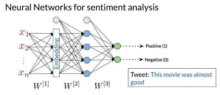
Neural Network predict tweets sentiment, structure:
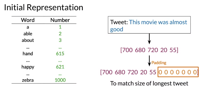
- Input is a vector of Integers, assign each word based on index from vocabulay and apply padding set length as maxlen of sentence of the tweet
- Embedding layer: transform the representation
- Hidden layer with a ReLU activation function
- output layer with softmax function that give probabilities for whether a tweet is positive or negative sentiment
This structure allow to predict complex tweets: 比如 “This movie was almost good”. 不能 classify correctly using simpler method 比如 Naive Bayes
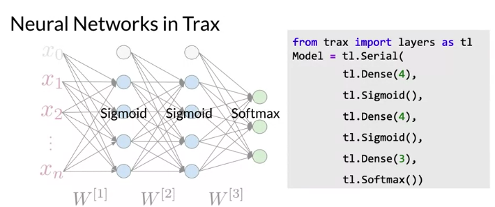
Trax
List the layer from left to right. Note Dense layer(fully-connected layer): A maps collections of R^m vectors to R^n, where n (= n_units) is fixed at layer creation time,. Fully computation is y = Wx + b. Generally followed by a non-linear activation function.
Advantage: (Trax is based on Tensorflow, use Tensorflow as a backend, also use JAX library to speed up computation)
- Run fast on CPUs, GPUs and TPUs(perform computations efficiently), don’t need to change a single line of code for running on CPU, GPU, TPU
- Run code fast (than tensorflow / PyTorch): Trax can run on-demand or preemptible Cloud without changing a single line of code
- allow parallel computing: allow model running on multiple machines or cores simultaneously
- Record algebraic computations for gradient evaluation, so they compute gradient automatically.
- Makes programmers efficient: Easy to Debug and understand (code structure like original paper)
Trax Development History: TensorFlow (2014-2015) -> Translate(2016, long time to train, not practical for anyone else other than Google) -> Tensor2Tensor(2017, userd by many large companies in the word. Complicated but not nice to learn, hard for new researchers) -> Trax
Trax: Deep Learning library with Clear Code and Speed
Some Resource
- Official Trax documentation maintained by the Google Brain team
- Trax source code on GitHub
- JAX library
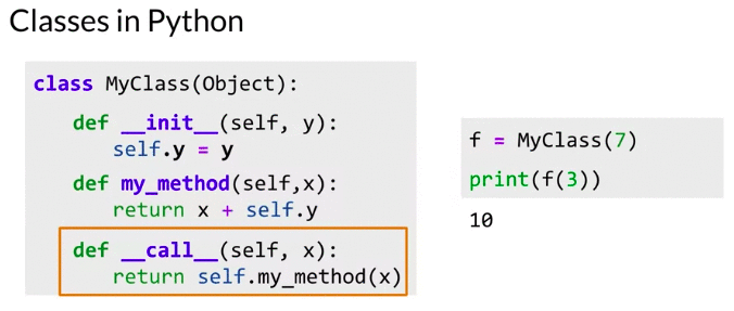
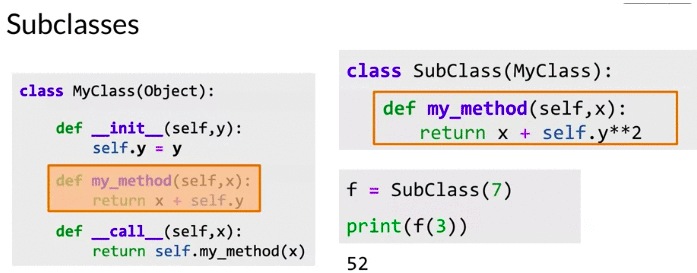
Python Class & Subclass(subclass can override method in super class )
Trax Layers
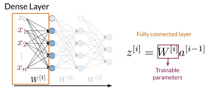
Dense Layer: The single inner product between trainable wights and input vector is called Dense layer computed as y = np.dot(x, w) 而不是 np.dot(w, x) 是为了方便计算
- The number of columns(second dimension) in the weight matrix is the number of units chosen for that dense layer. (output 的unit)
X = Input(shape= (3,))
X_out  = Dense(units = 4)(X)
model = Model(inputs = X, outputs = X_out)
print(model.summary())
# Layer (type)                 Output Shape              Param #

# =================================================================

# Input_17 (InputLayer)        [(None, 3)]         0

# _________________________________________________________________

# dense_11 (Dense)             (None, 4)           16

# =================================================================

# Total params: 16

# Trainable params: 16

# Non-trainable params: 0

e2 = model.layers[0].get_weights()
print(len(e2)) # 2, W and b

print(e2[0].shape) # (3, 4)


X = Input(shape= (2, 3))
X_out  = Dense(units = 4)(X)
model = Model(inputs = X, outputs = X_out)
print(model.summary())
# Layer (type)                 Output Shape              Param #

# =================================================================

# Input_17 (InputLayer)        [(None, 2, 3)]         0

# _________________________________________________________________

# dense_11 (Dense)             (None, 2, 4)           16

# =================================================================

# Total params: 16

# Trainable params: 16

# Non-trainable params: 0

e2 = model.layers[0].get_weights()
print(len(e2)) # 2, W and b

print(e2[0].shape) # (3, 4)
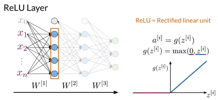
ReLU Layer: activation layer that follows a dense fully connected layer, and transforms any negative values to zero.
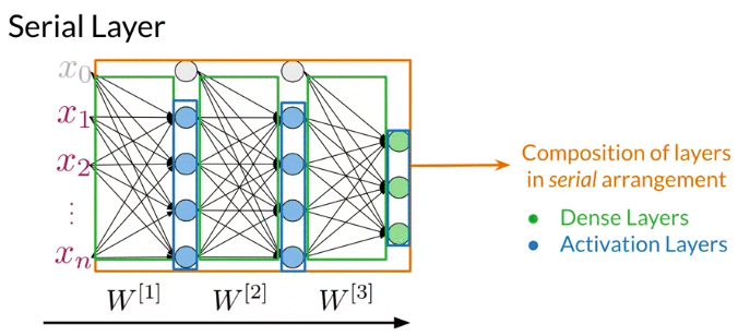
Serial Layer: a composition of sublayers layers that operates sequentially to perform the forward computation of entire model. Can think of serial layer as whole neural network model in one layer
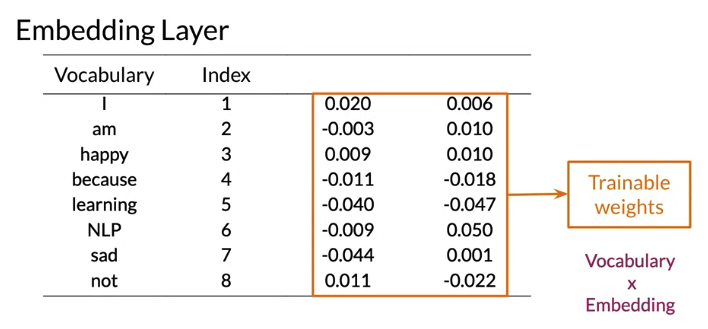
Embedding Layer: map words from vocabulary to representation of that word with determined dimension, 下面例子 embedding size = 2.
- In Trax, model learn representation of embedding that give the best performance.
- Size of weight =
Vocabulary size x # Embedding - size of embedding is hyperparameter in the model
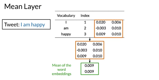
Mean Layer: Take means of each features from embedding. After mean layer, will have the same number of featurres as embedding size. Note: No trainable parameters because it’s only computing the mean of word embeddings
trax.layers.tl.Mean: Calculates means across an axis. Chooseaxis = 1(axis = 0is batch size)to get an average embedding vector (an embedding vector that is an average of all words in the vocabulary).
# Pretend the embedding matrix uses  2 elements for embedding the meaning of a word

# and has a vocabulary size of 3, So it has shape (2,3)

tmp_embed = np.array([[1,2,3,],
                    [4,5,6]
                   ])
print("The mean along axis 0 creates a vector whose length equals the vocabulary size")
display(np.mean(tmp_embed,axis=0)) # DeviceArray([2.5, 3.5, 4.5], dtype=float32)

print("The mean along axis 1 creates a vector whose length equals the number of elements in a word embedding")
display(np.mean(tmp_embed,axis=1)) # DeviceArray([2., 5.], dtype=float32)
- TrainTask:
trax.supervised.training.TrainTask(labeled_data, loss_layer, optimizer, lr_schedule=None, n_steps_per_checkpoint=100): A supervised task (labeled data + feedback mechanism) for training.initparameter 有- labeled_data: Iterator of batches of labeled data tuples. Each tuple has 1+ data (input value) tensors followed by 1 label (target value) tensor. All tensors are NumPy ndarrays or their JAX counterparts.
- n_steps_per_checkpoint: How many steps to run between checkpoints. 每run n_steps_per_checkpoint 会print出loss_layer,如果有eval_task, 同样也会run eval_task,然后print eval task metrics
- EvalTask,
EvalTask(labeled_data, metrics, metric_names=None, n_eval_batches=1)Labeled data plus scalar functions for (periodically) measuring a model.- labeled_data: Iterator of batches of labeled data tuples. Each tuple has 1+ data tensors (NumPy ndarrays) followed by 1 label (target value) tensor.
[tl.CrossEntropyLoss]
- labeled_data: Iterator of batches of labeled data tuples. Each tuple has 1+ data tensors (NumPy ndarrays) followed by 1 label (target value) tensor.
- Training.Loop:
Loop(model, task, eval_model=None, eval_task=None, output_dir=None, checkpoint_at=None, eval_at=None)Loop that can run for a given number of steps to train a supervised model. The typical supervised training process randomly initializes a model and updates its weights via feedback (loss-derived gradients) from a training task, by looping through batches of labeled data.
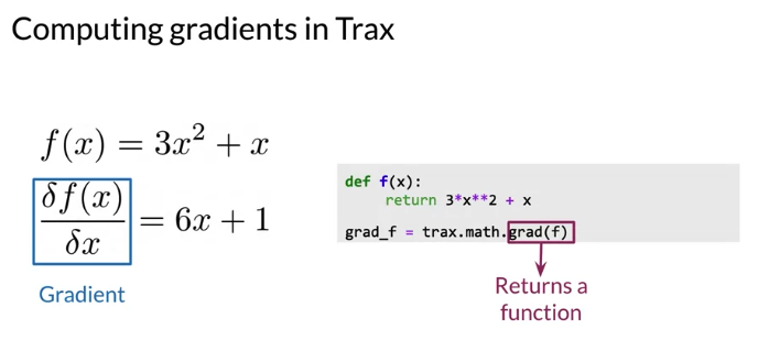
Gradient in Trax
- function
gradreturn a function that computes the gradients of f- allows much easier training
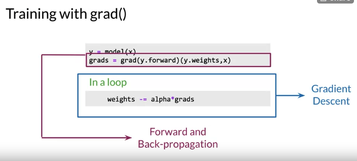
- forward and backward in a single line
- Notice the double parentheses, 第一个是 pass grad function, 第二个pass是arguments returned by grad
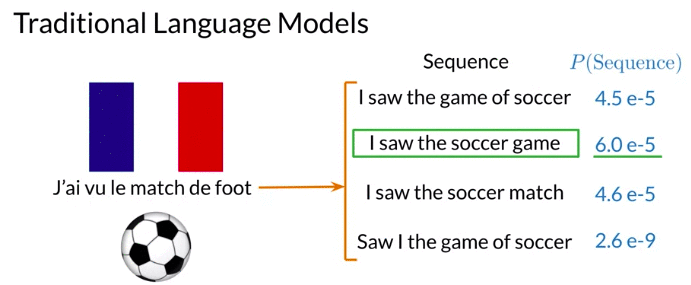
3.2 RNN for Language Modeling
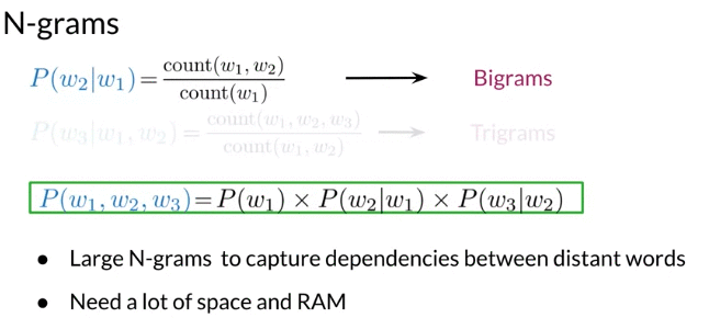
Problem with N-grams: for N grams, model have to account for conditional probabilites for long sequences, difficult to estimate for long corpora: Need a lot of space and RAM. e.g. if user download app, may not have enough space to store n-grams.
RNN
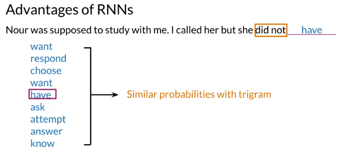
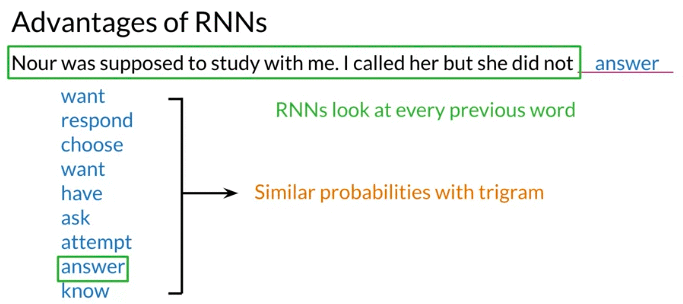
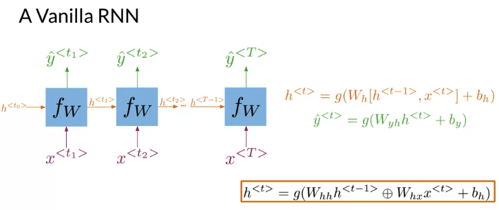
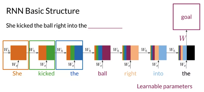
RNN: Looks at previous N words, propagate the information from the beginning to the end
e.g. 下面例子,tri-gram probabable choose “have”: because “did not have” is high probable in text corpus. But if choose “have” => sentence not make sense. If want to predict using n-gram, have to account 6-grams, impractical
- Each box represent the computation made at each steps and colors represent the information used for every computation. The computation at the last step have the information from all the words in the sentence
- Every word in the sequence is multiplied by the same weight \(W_x\), the information propagate from the beginning to the end is multiplied by \(W_h\).
- The block is repeated for every word in the sequence. The only learning parameters are \(W_x, W_h\). They compute values that are fed over and over again until the prediction is made.
Advantage of RNN
- RNN model relationships among distant word
- Note:An RNN would have the same number of parameters for word sequences of different lengths. (Computations share parameters)
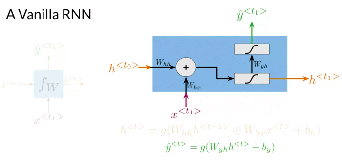
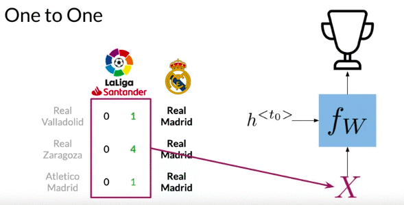
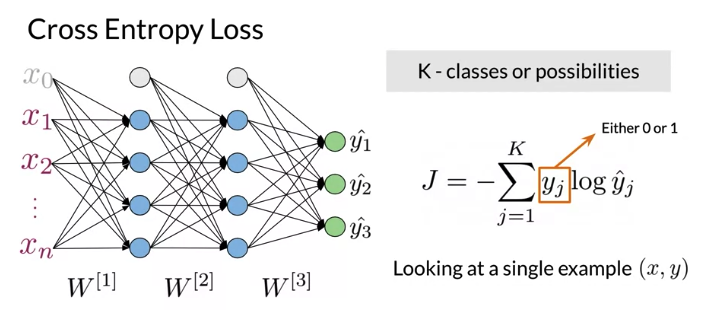
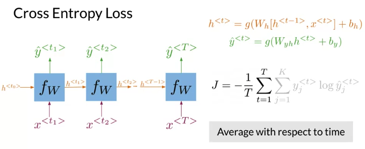
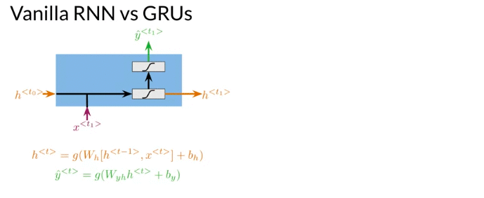
Many to Many architecture, at each time step, two inputs, x, hidden state h. Make a prediction \(\hat y\). Additionally, it propagate a new hidden state to the next time-step. The hidden state at every time t is computed with an activation function g. After computing the hidden state at time t, possible to get the prediction \(\hat y\) by using an activation function g
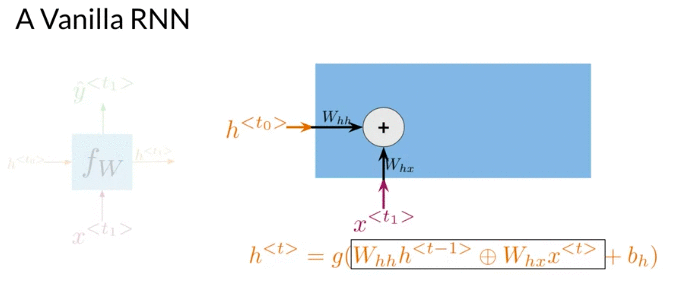
\[\begin{align} h^{<{t}>}& = g\left(W_h \left[ h^{<{t-1}>}, x^{<{t}>} \right] + b_h \right) \\ & = g\left(W_{hh} h^{<{t-1}>} \oplus W_{hx} x^{<{t}>} + b_h \right) \quad \oplus \text{sum up element-wise} \\ \end{align}\] \[W_h = \left[W_{hh} \mid W_{hx} \right] \quad \color{red}{\text{Horiztonal Stack}}\] \[\left[ h^{<{t-1}>}, x^{<{t}>} \right]= \left[ \frac{h^{<{t-1}>}}{x^{<{t}>}} \right]\] \[\hat y^{<{t}>} = g \left( W_{y_h} h^{<{t}>} + b_h \right)\]Many-to-many architecture
First step of the RNN
e.g. if \(h^{<{t}>}\) size is 4 x 1, \(x^{<{t}>}\) size is 10 x 1, what is the size of \(W_h\), given \(h^{<{t}>} = g\left(W_h \left[ h^{<{t-1}>}, x^{<{t}>} \right] + b_h \right)\)
Q: 4 x 14. In deep learning framework, it is 14 x 4
Application
One to One: Give lists of score from favorite team to predict the position of your team on the leaderboard
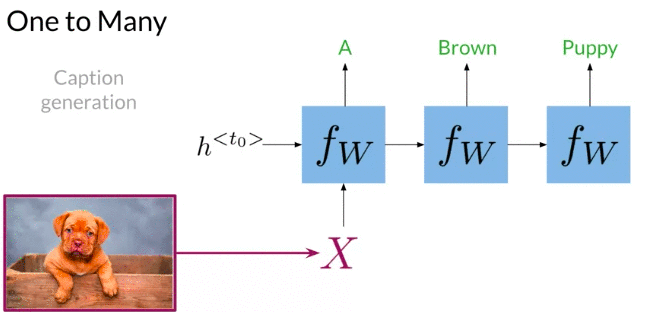
One to Many: Given picture => predict caption
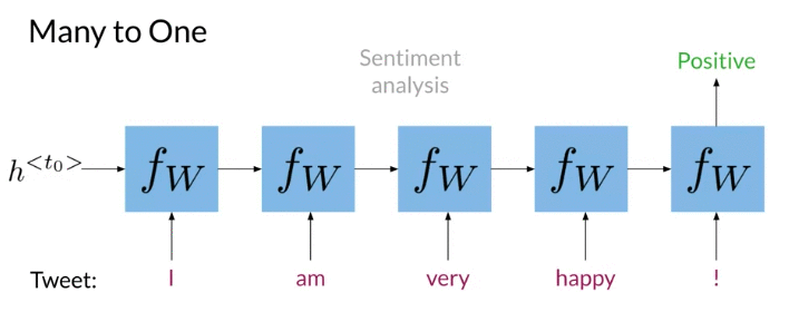
Many to One: Sentiment Analysis
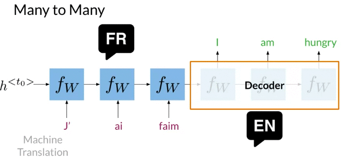
Many to Many: machine translation: encode and decoder architecture is popular for machine translation. First half doesn’t return output is called Encoder, because it encodes the sequences of words in a single representation that caputres the overall meaning of the sentence. Decoder generate a sequence of words in other language.
Cost Function
k: the number of category/class. \(y_j =\) 0 or 1 for each class, 比如下图output 3 classes
For RNN:
\(J = -\frac{1}{T} \sum_{t=1}^T \sum_{j=1}^K y_j^{<{t}>} log \hat y_j^{<{t}>}\), 与上面普通neural network cost function difference is summation over time T and division by the total number of steps T: is the average of the cross entropy loss function over time
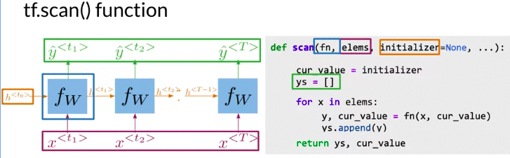
Scan Function
- Scan function is to take a function
fn( equivalent to 下图中的 \(f_w\)), and apply to all the elements from beginning to end in the listelems(\(x^{<{t_1}>}, x^{<{t_2}>} ... x^{<{T}>}\))) elemsis all the input through the time- Initializer (the hidden state \(h^{<{t_0}>}\)) is an optimal variable that could be used in the first computation of
fn(下图的中fn 是 \(f_W\)) - Function first initialize hidden states \(h^{<{t_0}>}\), set ys as an empty list
- For every x in the list of elements,
fnis called with x and the last hidden state as arguments, - For loop computes every time step for RNN, stores prediction value and hidden states
- Finally, function returns a list of predictions, and last hidden state
- Framework like Tensorflow need this type of abstraction in order to perform parallel computing and run on GPUs.
Advangtage of Scan function:
- Faster training
- Allow parallel computing
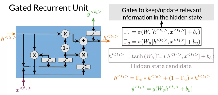
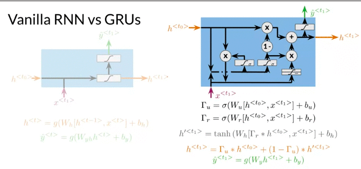
Gated Recurrent Units
- control how much information forget from the past and how much information to extract from current input.
- allow relevant information to be kept in the hidden states, even over long sequences. 比如下面例子,Ants learn Plural. GRU complete it by computing irrelevance and update gates. Can GRUS as Vanilla RNN with additional computations
- The first two computation in GRU are relevance gate \(\Gamma_r\), update gate \(\Gamma_u\) computed from sigmoid function. The output vectors of value are between 0 and 1. The output help determine which information from the previous hidden state is relevant and which values should be updated with current informations
- Update gate determines how much of information from the previous hidden state will be overwrited.
- \(h^{'<{t}>}\) is a hidden state candidate that could overwrite previus hidden state
- a prediction \(\hat y\) is computed using current hidden state
Vanilla RNN vs GRUs:
- Problem with Vanilla: update the hidden state at every time step, for a long sequences, information tends to vanish. So called vanishing gradients problem
- GRUs compute significantly more operations, can cause longer processing times and memory usage. GRUS help preserve important information for longer sequences by deciding how to update the hidden state.
mode = 'train'
vocab_size = 256
model_dimension = 512
n_layers = 2

GRU = tl.Serial(
      tl.ShiftRight(mode=mode), # Do remember to pass the mode parameter if you are using it for interence/test as default is train

      tl.Embedding(vocab_size=vocab_size, d_feature=model_dimension),

      [tl.GRU(n_units=model_dimension) for _ in range(n_layers)], # You can play around n_layers if you want to stack more GRU layers together

      tl.Dense(n_units=vocab_size),
      tl.LogSoftmax()
    )


def show_layers(model, layer_prefix="Serial.sublayers"):
    print(f"Total layers: {len(model.sublayers)}\n")
    for i in range(len(model.sublayers)):
        print('========')
        print(f'{layer_prefix}_{i}: {model.sublayers[i]}\n')

#show_layers(GRU)

#Total layers: 6

# ========

#  Serial.sublayers_0: ShiftRight(1)

# ========

# Serial.sublayers_1: Embedding_256_512

# ========

# Serial.sublayers_2: GRU_512

# ========

# Serial.sublayers_3: GRU_512

# ========

# Serial.sublayers_4: Dense_256

# ========
Deep Bidiretion RNN
e.g. 比如下面例子blank 来自于后下文
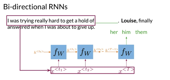
Could have another architecture where the information flow from end to beginning.
- Information flows from the past(from left to right) and from the future(from right to left) independently (acyclical graph)
- Get prediction \(\hat y\), have to start propagate information from both directions
- After compution all the hidden states for both directions, can get all of remaining predictions.
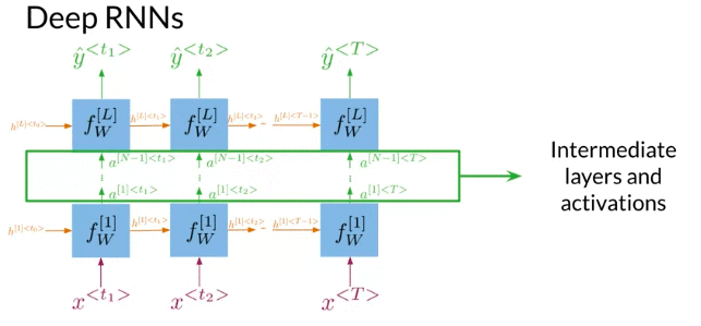
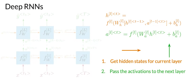
Deep RNNs are similar to deep neural networks. Deep RNN have a layer which takes input sequence x and multiple additional hidden layers. Like RNN stack together.
- Deep RNNs have more than one layer, which helps in complex tasks
- Get hidden states for current layer: At first progragate information through time.
- pass the activations to next layer. Go deeper in the network and repeat the process for each layer until get prediction
3.3 LSTMs and Named Entity Recognition
Simple RNN Advantages:
- Capture dependencies within a short range
- Takes up less RAM and space(lightweight) than other n-gram models
Simple RNN Disadvantages:
- Struggles with longer sequence
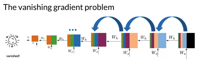
- Prone to vanishing or exploding gradients: This can arise due to the fact that RNN progagates information from the beginning of the sequence to the end.
- Starting with first words, the first values are computed(下图橙色框). Then it propagates some computed information takes the second word in the sequence, an gets new value(下图绿色框). Final steps, computations contain information from all the words in the sequence, then RNN predict next word.
- Notice: the information from first step doesn’t have much influence on the output. Orange portion from the first step decrease with each new step, and the computation at the first steps don’t have much influence on the cost function.
Vanishing/Exploding Gradient
Backprop: The derivatives from each layer are multiplied from back to front in order to compute the derivative of initial layer. The weights receive an update is proportional to the gradients with respect to the current weights of that time step. But in the network with many time steps or layers, gradient arrived back at early layers as the product of all the terms from the later layer -> make unstable situation. Especially if the values become so small -> no longer updates properly. For exploding gradients, work in opposite direction as updated weights become so large causing network to become unstable.(numerical overflow)
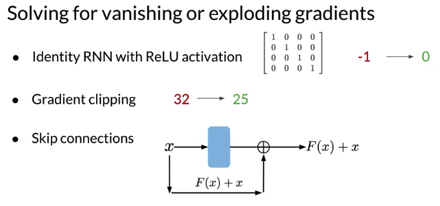
Solution:
- Identity RNN with ReLU activation: Initialize weights as indentity matrix: what it does, copy previous hidden state, add information from current inputs and replace any negative values with 0. Has effects of your network to stay close to the values in the indentity matrix which act like 1s during matrix multiplication
- only works for vanishing gradients, as derivatives of ReLu = 1 for all values greater than 0
- Gradient clippings: simply choose a relevant value that clip the gradients e.g. 25. Using this technique, any value grater than 25 will be clipped to 25
- works for exploding gradients. serves to limit the magnitute of gradients.
- Skip connections: provide a direct connection to earlier layers, effectively skips over activation functions, add values from initial inputs x to outputs, e.g. F(x) + x. so activations from eariler layers have more influence over the cost function
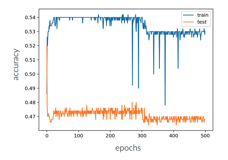
下图可能有vanishing gradient problem, because for a good model, performance should improve accuracy through time
LSTM
Application for LSTM
- Next-character prediction for email
- chatbots capable of remembering longer conversations
- music composition: consider music is built using long sequences of notes, much like text uses long sequences of words
- image caption
- speech recognition
LSTM: special variety of RNN handle entire sequences of data by learning when to remember and when to forget, similar to GRU
- cell state \(c^{<{t_0}>}\): can think of cell as memory of your network, carrying all the relevant information down the sequence.
- As cell travels, each gate adds or removes information from cell state
- Three hidden states gates. Gates allows gradients to flow unchanged. -> so vanishing/exploding gradient is mitigated
- Forget gate decides what to keep
- Input gate decides what to add
- Output gate decides what the next hidden state will be
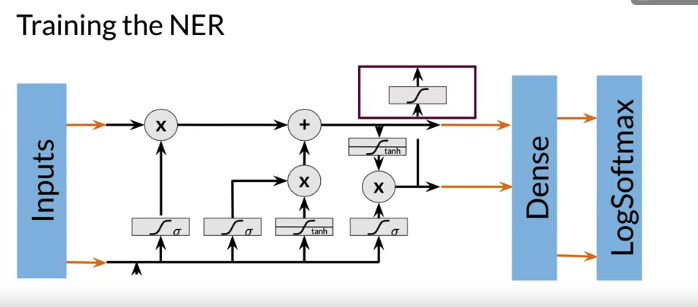
Structure:
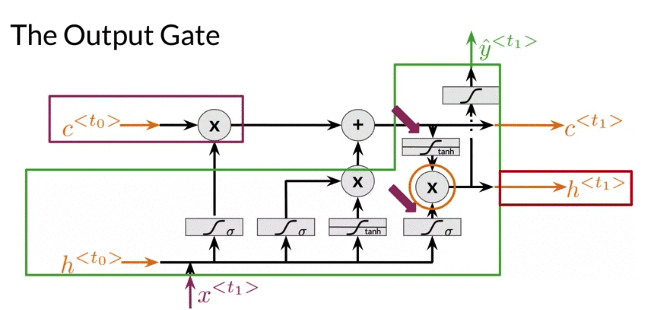
Note: The tanh layer’s output (between -1 and 1) is multiplied element-wise by the sigmoid layer’s output /update gate. ensuring an even flow through the LSTM unit. This prevents any of the values from the current inputs from becoming so large that they make the other values insignificant. Ensures the values in your network stay numerically stable, - \(h^{'<{t}>}\) and \(\Gamma_u\); \(tanh\left(h^{<{t}>}\right)\) and \(\Gamma_o\) are all element-wise product
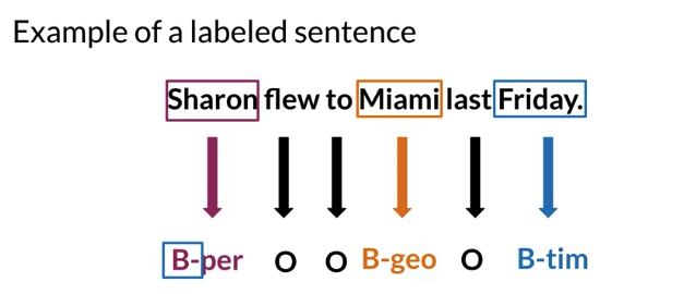
NER
NER: Named Entity Recognition: fast and efficient way to scan text for certain kinds of information.
- NERs sytems locate and extract named entities from text.
- Name entities can be a place, an organization or a person’s name, can even be times and dates.

- B dashes denotes entity
- All other words are classified O
Application:
- Search engine efficiency: NER models scan millions of websites once and stores the entities as indentified in the process. Then tag from your search query simply match against website tags.
- Recommendation engines: tags extracted from your history and compared to similar user histories then recommend things you might want to check out
- Customer service: match customer to an appropriate customer service agents. works similarly to a phone tree where prompted to provide some information about your request. e.g. use an app to communicate with your car insurance company, 需要provide some spoken information. then match to appropriate agents
- Automatic trading: build a web scraper to get the articles of the names of certain CEOs, Stocks, or cryptocurrencies. Then feed those article into a sentiment classification system and make your trade accordingly
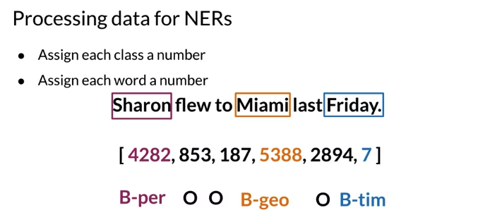
Training NERS: Data Processing
- Assign each entity class to a unique number. e.g. person name = 1, geographical location = 2, time indicator = 3
- Assign each word a number that corresponds to its assigned entity class. O 表示 a failure or unrecognized word. Numbers are random and assigned when you process your data. Each sequence is transformed into an array of numbers where each number 表示 index of the labeled word
- papdding: LSTM require all sequences are the same length. Can set length of sequnces to a certain number and add generic
<PAD>token to fill all empty spaces.
Traing the NER:
- Create a tensor for each input and corresponding number
- Create a data generator and put them in a batch, batch size normally power of 2, speed up processing time considerably -> 64, 128, 256, 512…
- Feed it into an LSTM unit
- Run the output through a dense layer (Linear operation on the input vectors) or fully connected layer
- Predict using a log softmax over K classes (K: the number of possible output), log softmax gets better numerical performance and gradients optimization than softmax
tl.Serial(
    tl.Embedding(),
    tl.LSTM(),
    tl.Dense(),
    tl.LogSoftmax()
)
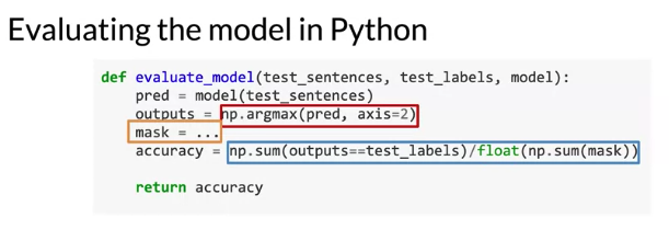
Evaluate the model
- Pass test set through the model
- Get arg max across the prediction array, 下面
np.argmaxtakes an axis parameter. To implement it accurately, need to consider the dimension of array - make sure arrays are padded using
<PAD>token, which makes arrays the same length - Compare outputs against test labels to see how accurate model is
Note: When you pad your tokens, you should mask them before computing accuracy.
下面code, mask variable is any token IDs that need to be skipped over during evaluation. One token need to skip is <PAD> token
Some Useful Link
Intro to optimization in deep learning: Gradient Descent
3.4 Siamese Network
It’s made up two identical neural networks which are merged at the end. Used as Indentify similarity between things
e.g. Comparing meaning not the same as compare words
- How old are you = what is your age
- Where are you from \(\neq\) where are you going. Although first three words are the same
Application:
- Question duplicates: Stackoverflow, Quera check your questions if exist before post
- Handwritten checks: determine if two signatures are the same or not
- Search engine queries: to predict whether a new query is similar to the one that was already executed
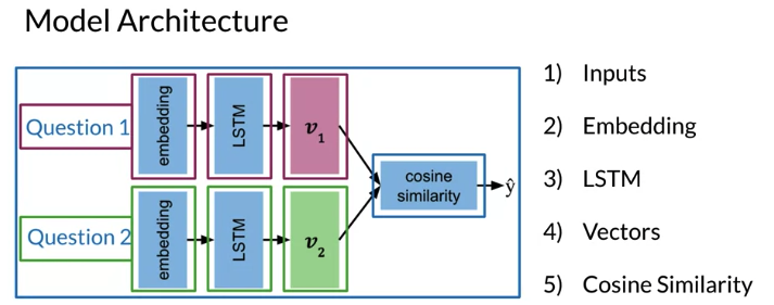
Architecture
- Both network have a identical sub network. 并且sub networks share identical parameters. Learned parameters of each sub-network are exactly the same. Networks are merged together through a Dense layer to produce a final output or similarity score
- Each network output a vector, one for each questions.
- Cosine similarity tells how similar they are, \(\hat y\) a value between -1 and 1
- if \(\hat y \leq \tau\) means input questions are different. if \(\hat y > \tau\) means input questions are the same. \(\tau\) is a parameter that choose how often want to interpret cosine similarity to indicate two questions are similar. Higher threshold means only very similar sentences is considered similar
下面是一个example, not all Siamese network contain LSTM.
def normalize(x):
    print("x square", np.sqrt(np.sum(x * x, axis=-1, keepdims=True)))
    return x / np.sqrt(np.sum(x * x, axis=-1, keepdims=True))

vocab_size = 500
model_dimension = 128

# Define the LSTM model
LSTM = tl.Serial(
        tl.Embedding(vocab_size=vocab_size, d_feature=model_dimension),
        tl.LSTM(model_dimension),
        tl.Mean(axis=1),
        tl.Fn('Normalize', lambda x: normalize(x))
    )

# Use the Parallel combinator to create a Siamese model out of the LSTM

Siamese = tl.Parallel(LSTM, LSTM)
def show_layers(model, layer_prefix):
    print(f"Total layers: {len(model.sublayers)}\n")
    for i in range(len(model.sublayers)):
        print('========')
        print(f'{layer_prefix}_{i}: {model.sublayers[i]}\n')

print('Siamese model:\n')
show_layers(Siamese, 'Parallel.sublayers')

#Siamese model:

# Total layers: 2

# ========
# Parallel.sublayers_0: Serial[

#  Embedding_500_128

#  LSTM_128

#  Mean

#  Normalize

# ]

# ========


# Parallel.sublayers_1: Serial[

#  Embedding_500_128

#  LSTM_128

#  Mean

#  Normalize

# ]
Cost Function
- Anchor: the first question e.g. “How old are you”
- positive questions: have the same meaning as anchor, cosine similarity close to 1
- negative questions: not have the same meaning as anchor, cosine similarity close to -1
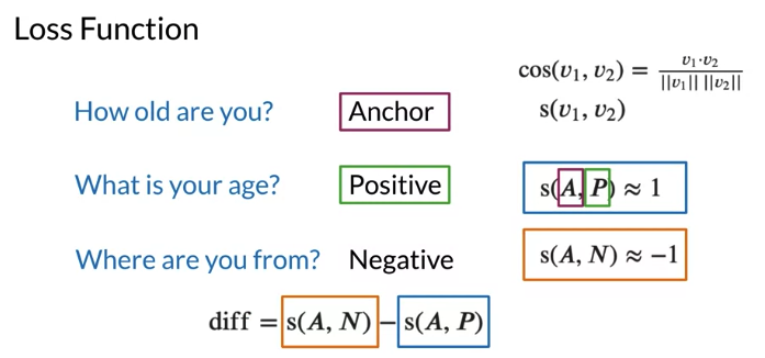
s(v1, v2) is similarity metric(cosine similarity), could be distance metrics d(v1, v2) such as ecludian distance
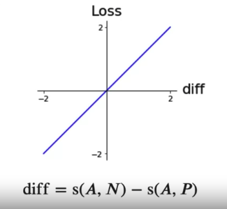
loss function allow whether model do well. When difference betwen s(A,N) and s(A,P) bigger or smaller along x-axis, loss bigger or smaller along the y-axis. Minimizing loss in training-> minimize this difference. But below loss function when loss < 0, still update maybe update to a worse weight which is not good
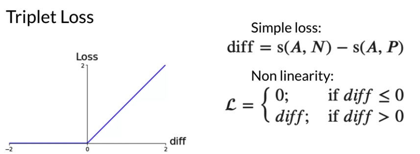
To fix above problem, when model do a good job, no need to update the weight. Modify if loss < 0, then loss = 0. When the loss is zero, we are not asking model to update the weight. But if predict all s(A,N) and s(A,P) pair as zero, loss function could not update
We want the loss to be negative for model performing well. 如果difference is just less than zero, want model to still learn and ask to predict a wider difference, can shift the loss function a little to the left. margin refer as Alpha. Loss function shift to left by \(\alpha\). So if difference less than 0 but small in magnitute, loss greater than 0 and still can learn to improve
- s could be similarity function or Distance Metric(e.g. Euclidean distance) measurement. A distance metric is the mirror of a simlarity metric. A simlarity metric can be drived from a distance metric
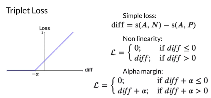
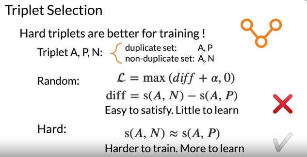
Triplet Loss
\[L = \begin{cases}0; \quad \text{if diff } + \alpha \leq 0 \\[2ex] diff; \, \text{if diff } + \alpha > 0 \\ \end{cases}\] \[L\left(A, P, N \right) = max\left(diff + \alpha, 0 \right)\]Triplet Selection
- Firstly, select pair of duplicate questions as anchor and positive
- Secondly, select a question is difference meaning from the anchor, to form anchor and negative pair
- 错误的方式是: select triplet random: 很可能select non-duplicative pair A and N, where loss equal to 0. Loss is zero whenever model correctly predict A and P more similar to A and N. When
loss = 0, network little to learn from triplet. - Hard Triplet: are more difficult to train. Hard triplets 是similarity between anchor and negative very close to, but still smaller than similarity between anchor and positive. \(S\left(A, N \right) \approx S\left(A, P \right)\) When model encounter hard triplet, algorithm need to adjust its weight so that yield similairty line up with labels
- By selecting hard triplets, trainning focus are doing better on difficult cases which 也许会predict incorrectly
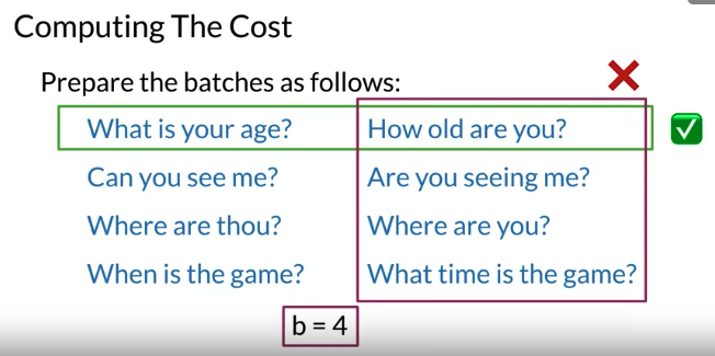
Compute Cost Function
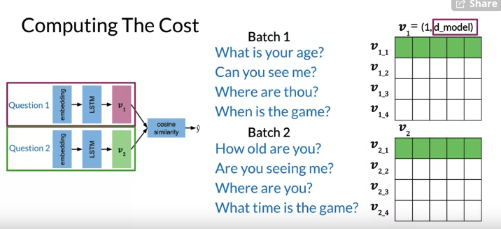
Use b as batch size, 如下图每一行,是duplicate, 每一个column 没有duplicate
- vector \(v_{1}\), #row = batch sizes
- \(v_{1}\) #columns is the number of embedding layer(
d_model). - \(v_{1,1}\) is a duplicate of \(v_{2_1}\), but \(v_{1_1,}\) is not a duplicates of any other row in \(v_{1}\) e,g, \(v_{1_2}, v_{1_3}\)
may get similarity as 下图左侧的matrix
- Diagonal is the key features, These values are the similarities for positive examples, question duplicates. 通常diagonal 数比不是在diagonal的数要大, because expect duplicates have higher similarity than non-duplicates.
- upper right, lower left -> similarity for all negative examples. most number are lower than similarities along the diagonal
- 注意 negative example question pairs still have similarity 大于0, 虽然similarity range 从-1 到1,但不意味着大于0 表示duplicates 或小于表示non-duplicated. Really matter is to find duplicates have a higher similarity relative to non-duplicated.
- Creating pairs like this removing the need for additional non-duplicate example and input data. Insteading of sets up specific bathchs with negative examples, model can learn from existing questions duplicates batches.
Overall Cost Function
\[\begin{align}J &= \sum_{i=1}^{m} L\left(A^{\left(i\right)}, P^{\left(i\right)}, N^{\left(i\right)} \right) =\sum_{i=1}^{m} max\left(diff + \alpha, 0 \right) \\ &= \sum_{i=1}^{m} max\left(s\left(A^{\left(i\right)}, N^{\left(i\right)} \right) - s\left(A^{\left(i\right)}, P^{\left(i\right)}\right) + \alpha, 0 \right) \\& \color{blue}{\text{i refer to a specific training example and there are m observations}}\end{align}\]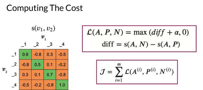
- Mean negative: mean of off-diagonal values in each row(mean of the similarity of negative examples, not mean of negative number in a row). 比如第一行 (-0.8 + 0.3 - 0.5)/3
- Closest negative: off diagonal value closest to(but less than) the value on diagonal in each row. By choosing this, force model to learn what diffferentiates these examples and drive those similarity values further apart through training. 比如第一行选取0.3: meaning a similarity of 0.3 has the most to offer model in terms of learning opportunity
In order to minimize the loss, you want \(diff + \alpha \leq 0\),
- Loss 1: using mean negative replace similarity of A and N, help model converge faster during training by reducing noise. Reduce noise by trainning on average of several observations rather than training model on each of these off-diagonal examples.
- Why reduce noise? We define noise to be a small value that from a distribution that is centered arund 0. So the average of several noise is centered around 0.(Cancel out individual noise from those observations)
- Loss 2: create a slightly large penalty by diminishing the effects of more negative similarity of A and N. can think of closest negative as finding negative example that results in smallest difference between two cosine similarity(Positive, Negative). Then add small difference to alpha, able to generate the largest loss among all of other examples in that row -> make the model update weights more
One Shot Learning
Classification vs One Shot Learning
- Classification: classify as 1 of K classes, probably use softmax function at the end to find maximum prabability. 比如k=10, 如果k增加一个类别, expensive to retrain the model. Besides unless you have many examples for the class. model training won’t work well
- One Shot Learning: one shot learning is to be able to classify new classes without retraining any models. You only need to learn the similarity function once. Then can test similarity score against some threshold to see if they are the same. Problem changes to determine which class to measure similarity between two classes
- 比如下面的例子,比如银行签字,每次有新的签名, can’t retrain entire system. Instead, just learn a similarity -> identify whether two signature are the same or not.
- If \(\text{similarity score} > \tau\) indicates the same
- If \(\text{similarity score} \leq \tau\) indicates the same
Training / Testing
- prepare batches with batch size = b. Corresponding questions from each batch are duplicate(batch 1 和 batch 2第一行是duplicate). No duplicates within an indiivual batch(比如batch 1 第一行和第二行不是duplicate).
- Use these inputs t get outputs vectors for each batch (Embedding -> LSTM -> Vectors -> Cosine Similarity). Note two subnetworks have identical parameters so only train one set, then shared by both
- Note: \(\tau\) and margin \(\alpha\) from loss function are tunable hyperparameter
- When testing model, perform one-shot learning.
- Convert each input an an array of numbers
- Feed arrays into model
- Compare \(v_1, v_2\) using cosine similarity
- Test against a threshold \(\tau\). If similarity greater than \(\tau\), questions are classified as duplicates
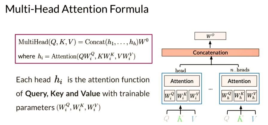
4.1 Attention Model
Alignment
- Many lanuage don’t translate exactly into another language. To align words correctly, need to add a attention layer to help the decoder understand which inputs are more important.
- The attention mechanism solves for longer input sequences by giving more weight to more important words.. More weight -> More influence for decoder output
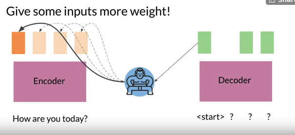
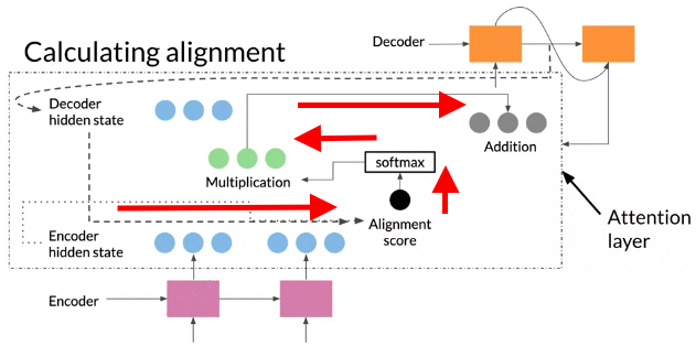
- Get all hidden states ready for encoder and first hidden states for decoder. 比如下面例子,encoder 两个hidden states, decoder一个
- Calculate Alignment Score: score each of encoder hidden state by 计算 compute dot product between Query and Key to get alignment Score . higher score->more influence of this hidden state activation for output.
- Run scores through softmax, each score is between 0 and 1, then give attention distribution.
- Take each encoder hidden state, multiply by its softmax score, -> alignment vector Z
- adding up everything alignment vector(add up weighted sum) to context vector -> context vector is feeded into decoder
RNN Disadvantage
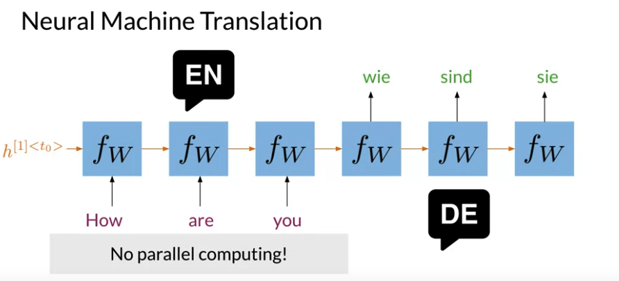
- RNN parallel computing diffcult to implement No parallel computing.
- The more for input, the more time process that sentence
- For long sequence in RNNs there is loss of information. LSTM and GRUS help a little(stop working well when process long sequence)
- In RNNs, problem of vanishing gradients
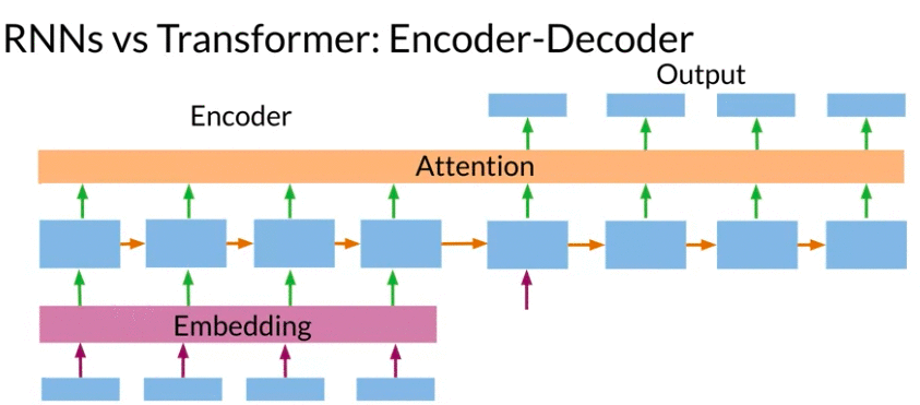
Transformers help with all of the above
Neural machine translation use neural network artchitecture: Both Encoder and Decoder take sequential steps.
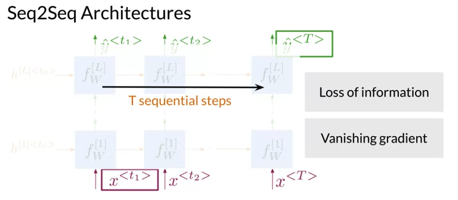
Seq2Seq Architecture:
- For large sequences: information tend to loss within the network, vanishing gradients problem.
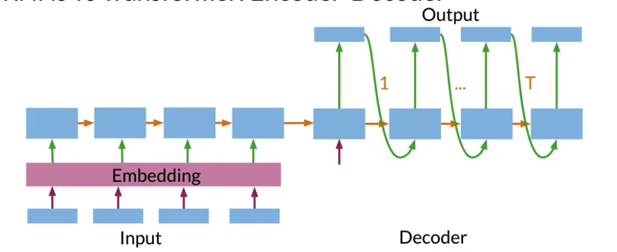
Conventional Encoder - Decoder Architecture
Query, Key, Value
- Encoder-Decoder attention, the queries are decoder states from the previous layer, keys and values and the encoder states.
- Self-Attentive: Query, Key, Value are all three of them the same, they are the outputs of the previous encoder layers(all bottom layers). Each position in the encoder can get attention score from every position in the previous encoder layer.
- Causal Attention/Masked self-Attention: all queries, keys, and values come from the previous layer. The self-attention decoder allows each position to attend each position up to and including that position
Then all these queries, keys, values(Two are the same or all are the same) through different Dense layer to form different representation
More Graghs/Explanations at geeksforgeeks
Self Attention
Dot-Product Attention
Self Attention(One-head attention)
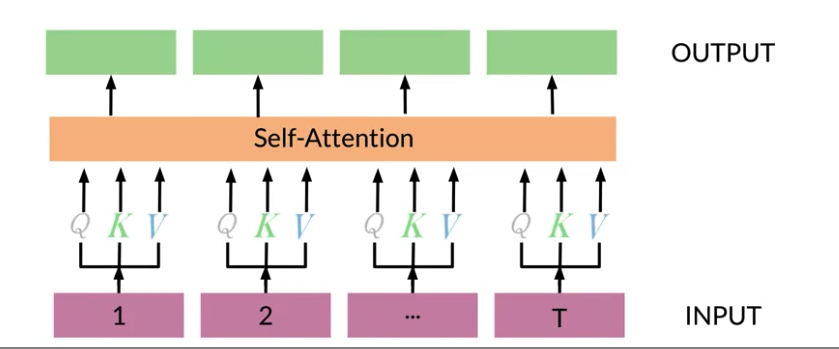
Dot-product Attention is essential for Transformer
- The queries by Keys matrix is called attention weights: how much each key similar to each query
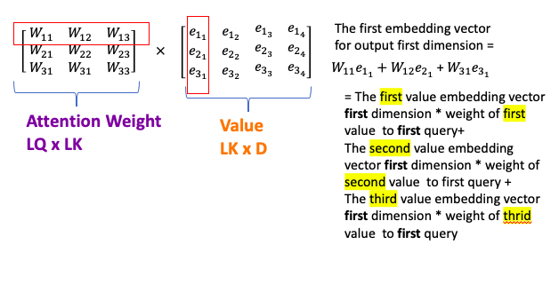
Math
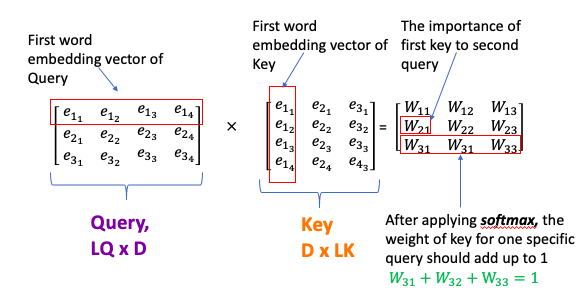
- pass encoder input vector through a Dense Layer to get Queries, Keys, and Values( same as multiply encoder with three weights \(W^Q, W^K, W^V\))
- Query: Shape: \(L_Q\) by D (can from input text or output label text)
- think of D is the embedding dimension of word embedding, \(L_K\): the length of German sentence
- Keys: Shape: \(L_K\) by D
- think of keys D is the embedding dimension of word embedding, \(L_K\): the length of English sentence
- Often Values and Keys are the same two copies
- Values: Shape: \(L_K\) by D
- Query: Shape: \(L_Q\) by D (can from input text or output label text)
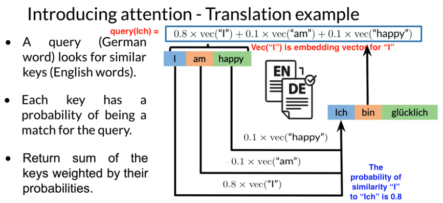
- Query assign each Key a probability using dot product if dot product large -> Q and K are similar. This allow the model to focus on the right place when translating each word
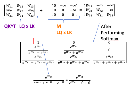
- Attenion weights: \(W_A = softmax\left( \frac{QK^T}{ \sqrt{d_k} }\right)\), shape is \(L_Q x L_K\). 每个key-query pair gets a probability
- divide the score by \(d_k\). The reason is if the dot products become large, this causes some self-attention scores to be very small after we apply softmax function in the future, and may cause gradients from the function to be extremly small. This leads to having more stable gradients
- Weights or Scores 表示relative importance of Keys for specific Query. Attention weights can be understood as alignments score.
- However, similarity number not add up to 1, cannot be used as probabilities. Solution: use softmax turn attention weights to probability
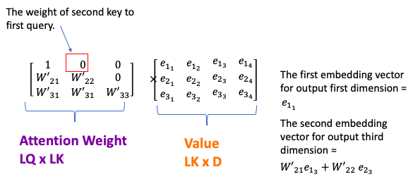
- Finally, multiply these probabilites with Values, get weighted sum of sequence(attention result/context vector). weight each value \(v_i\) by the probability that key \(k_i\) matches the query.
- Attention mechansim calculates dynamic or alignments weights 表示 relative importance of the inputs(Keys) in sequence for particular output (Queries). Multiply dynamic weights or alignments with input sequences(Values) to get a single context vector
- GPUs and TPUs is used for speed-up matrix multiplications
def DotProductAttention(query, key, value, mask, scale=True):
    # query (numpy.ndarray): array of query representations with shape (L_q by d)

    #key (numpy.ndarray): array of key representations with shape (L_k by d)

    #value (numpy.ndarray): array of value representations with shape (L_k by d) where L_v = L_k

    # mask (numpy.ndarray): attention-mask, gates attention with shape (L_q by L_k)

    # scale (bool): whether to scale the dot product of the query and transposed key


    assert query.shape[-1] == key.shape[-1] == value.shape[-1], "Embedding dimensions of q, k, v aren't all the same"

    if scale:
        depth = query.shape[-1]
    else:
        depth = 1

    dots = np.matmul(query, np.swapaxes(key, -1, -2)) / np.sqrt(depth)
    if mask is not None:
        dots = np.where(mask, dots, np.full_like(dots, -1e9))

    # Use scipy.special.logsumexp of masked_qkT to avoid underflow by division by large number

    # Note: softmax = e^(dots - logaddexp(dots)) = E^dots / sumexp(dots)

    logsumexp = scipy.special.logsumexp(dots, axis=-1, keepdims=True) #log of the sum of exponentials of input elements.

    dots = np.exp(dots - logsumexp)

    # Multiply dots by value to get self-attention

    attention = np.matmul(dots, value)
    return attention
Causal Attention
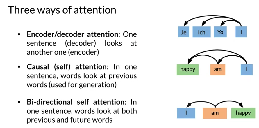
Three ways of Attention
- Encoder/decoder Attention: One sentence(decoder) looks at another one(encoder) German attends to English
- Causal (self) attention: In one sentence, words look at previous words(used for generation text/summary). 比如 “I am happy” happy look at “I” 和 “am”
- Bi-directional self attention: In one sentence, words look at both previous and future words (used in Bert/T5)
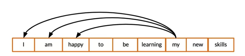
Causal attention: also called masked-self attention
- Queries/Keys are words from the same sentence(That’s why called self-attention). It is used in language models where try to generate sentences.
- 比如下面例子,after generating “my”, model may look at vector “I” to retrieve more information
- Query seach among past words only
- Causal attention cannot attend words in future . 因为future word还没有generated yet
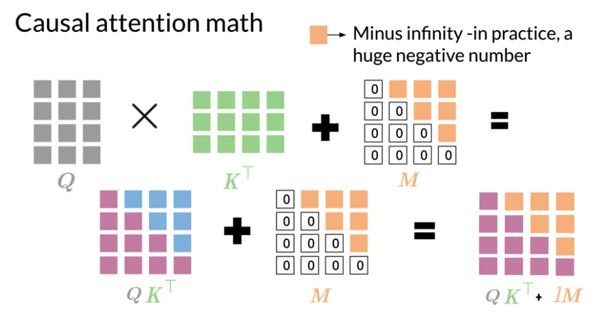
Math:
- \(softmax\left( QK^T \right)\) shape is \(L_Q\) by \(L_K\), allow model attend words in future
- add mask(a constant triangular matrix, has 0 on diagonal and below it, \(-\infty\) on other places ) to weights \(QK^T\)
- \(softmax\left( QK^T + M \right)\). Adding M let queries attending words in the past untouched. All other values become \(-\infty\). After softmax, all \(-\infty\) become to 0(exponential of \(-\infty\) equal 0) -> prevent words from attending to future
#Create Mask Matrices M

LQ = 10
LK = 10
M = np.tril(np.ones((1, LQ, LK), dtype=np.bool_), k=0)
Multi-headed Attention
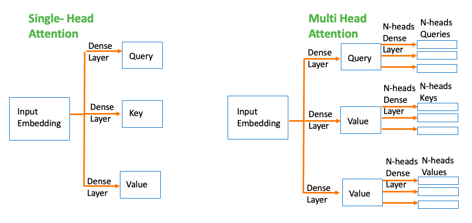
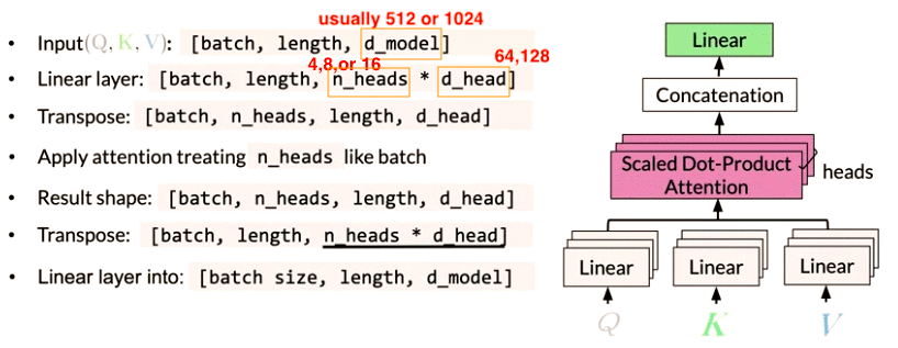
1 - create embedding for input words, run through Dense Layer to get Key, Value and Query. (Depending on the model structure, Dense Layer maybe the same for Key, Value,and Queries, so just three copies of the same matrices) input size is [batch, length, d_model]
2 - Initialize 3 x n_heads different weight matrics for each head of, Queries, Keys and Values, e.g. \(W_h^Q\) is for h-th head queries weighted matrix
- Each head uses individually different linear transformation(Dense layer) to represent word
3 - multiply input with each of weight matrics parallel (same as pass to n_heads Dense layer independently)
- Q mutiply \(W_i^Q\) to get ith head Query matrix \(Q_i\)
- K mutiply \(W_i^K\) to get ith head Key matrix \(K_i\)
- V mutiply \(W_i^V\) to get ith head Value matrix \(V_i\)
n_headis the parallel attention head.d_headis dimensionality for each head.- separate head don’t interact with each other
- Different heads can learn different relationships between words
4 - Apply dot product attention mechanism to these Query, Key, Value matrices and tread n_heads like batch parallel, and get result matrices \(Z_i\): i-th headed attention result
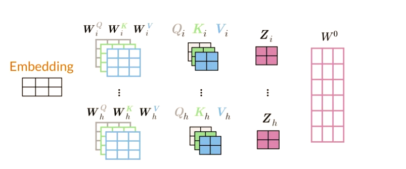
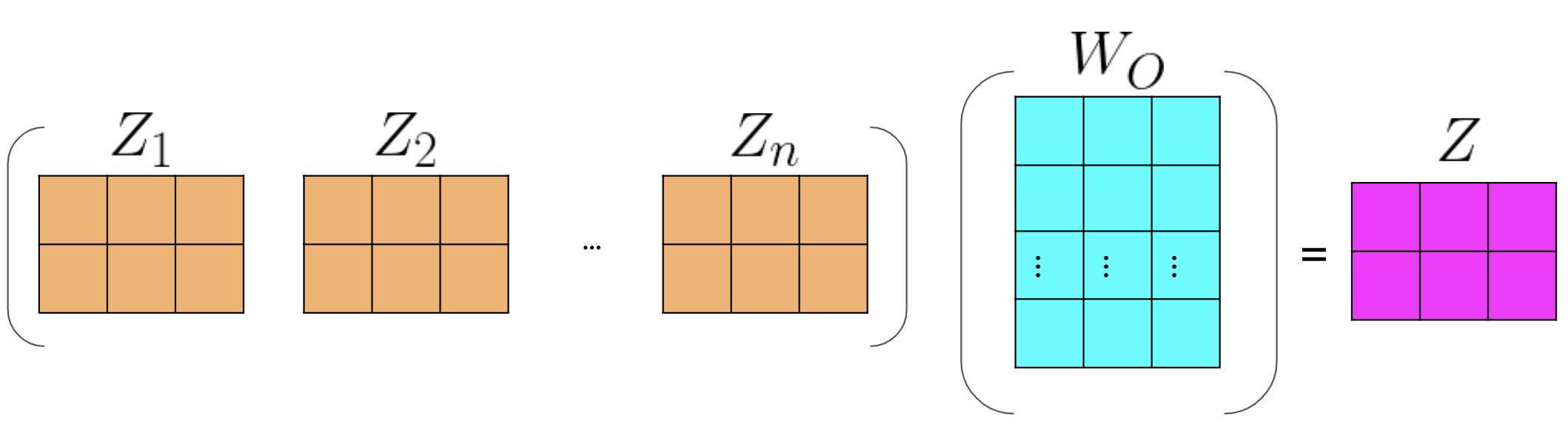
6 - concatenate the output matrix obtained from each attention heads and dot product with the weight \(W_O\) to generate the output Z of the multi-headed attention layer.
- Final Dense layer make different heads into a joint representation
A multi-headed model jointly attends to information from different representation at different positions over the projected versions of queries, keys and values.
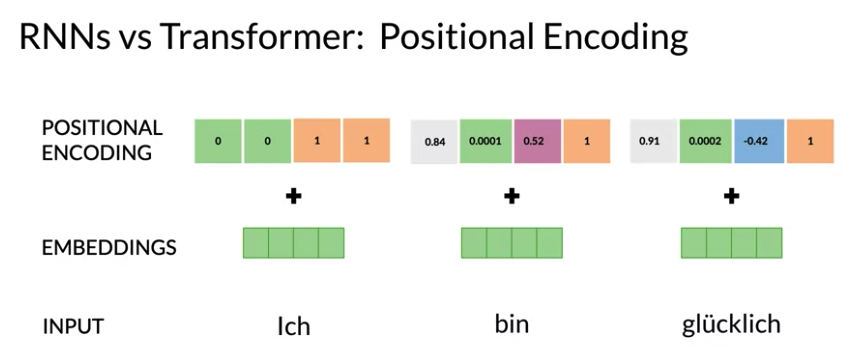
Position Encoding
Embed the words, then create vectors representing each word’s position in each sentence \(\in \{ 0, 1, 2, \ldots , K \} = \text{range(max_len)}\), where max_len = K+1
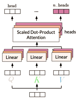
- Multiheaded attention: parallel self-attention layers(called heads). These heads are further concatenated to produce a single output, which emulates the recurrence sequence effect with attention
- Unlike recurrent layer, multi-headed attention computes the inputs in the sequence independently then allows to parallelize the computation. But fail to model the sequential information for a given sequence, that’s why need positional encoding stage into the transformer model
- Positional Encoding: encodes each input position in the sequence(since word order and position is important for language) to retain the positional information. The positional encoding output values to be added to the embeddings. So every word given to the model, have some of information about its order and position. 下面例子中 a positional encoding vector for each word ich, bin which will tell respective position.
- Position Encoding: add embedding the information about position. The information is to learn vector representing
{0,1,2,...k}- The embedding first word will get added with vector representing one, The embedding second word will get added with vector representing two, produce positional input embedding
Positional Encoding
def PositionalEncoder(vocab_size, d_model, dropout, max_len, mode):
    # 1. takes a block of text as input,

    # 2. embeds the words in that text, and

    #  3. adds positional encoding,

    #   i.e. associates a number in range(max_len) with

    #   each word in each sentence of embedded input text


    return [
        # Add embedding layer of dimension (vocab_size, d_model)

        tl.Embedding(vocab_size, d_model),
        # Use dropout with rate and mode specified

        tl.Dropout(rate=dropout, mode=mode),
        # Add positional encoding layer with maximum input length and mode specified

        tl.PositionalEncoding(max_len=max_len, mode=mode)]
4.2 Neural Machine Translation
Seq2Seq
- take one sequence of items such as words, and output another sequence.
- Map variable-length of sequence to a fixed-length memory. The inputs and outputs length 不一定一样
- In Seq2Seq model, LSTMs and GRUs are typically used to overcome the vanishing gradient problem
- Encode-Decoder:
- Encoder takes the input one step at a time, collects information for inputs then move it fowward by hidden state
- 橘色框 encoders final hidden states, all the information collected from each input step before feeding into the decoder. The final hidden states provide initial states for decoder to begin predicting the sequence.
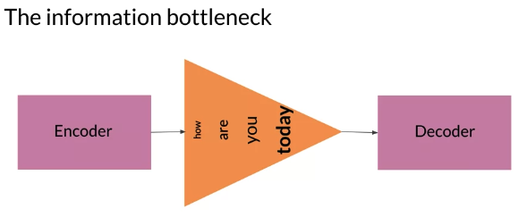
- Shortcomings of traditional Seq2Seq with LSTM: Information bottleneck
- 因为是Seq2seq (Encoder hidden states) uses a fixed length memory. longer sequence become problematic -> lower performance
- Later input steps in the sequence are given more importance. 比如下图中的today
One Vector per word: give each word a vector for individual information instead of smash all into one big vector. Flaw: How build a time/memory efficient model that predicts accurately from a long sequence.
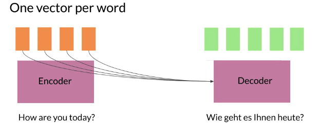
Solution: Focus attention in the right place:
- Prevent sequence overload by giving the model a way to focus on the likeliest words at each step. can think of a new layer to process this information.
- Do this by providing the information specific to each input word
The sequential nature of models (RNNs, LSTMs, GRUs) does not allow for parallelization within training examples, which becomes critical at longer sequence lengths, as memory constraints limit batching across examples. Have to wait until the initial computations are complete. This is not good
- it will take a long time for you to process it
- you will lose a good amount of information mentioned earlier in the text as you approach the end.
Therefore, attention mechanisms have become critical for sequence modeling in various tasks, allowing modeling of dependencies without caring too much about their distance in the input or output sequences.
#
Machine Translation Setup
- keep track of index mappings with word2ind and ind2word dictionaryie
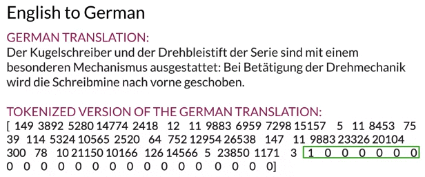
- use start-of
<SOS>and end-of<EOS>(1) sequence tokens
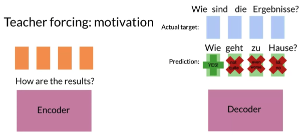
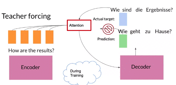
Teacher Forcing
- Teacher forcing use the ground truth or the actual outputs from decoder feed to next decoder layer as input instead of predicted value during training
- Teacher forcing yields faster, faster convergerence, more accurate training
e.g. In a sequence model, each wrong prediction make the following predictions even less likely to be correct..
NMT with Attension
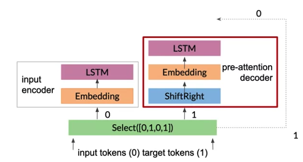
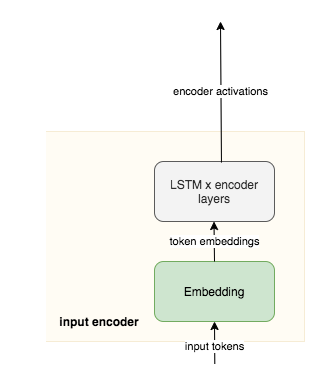
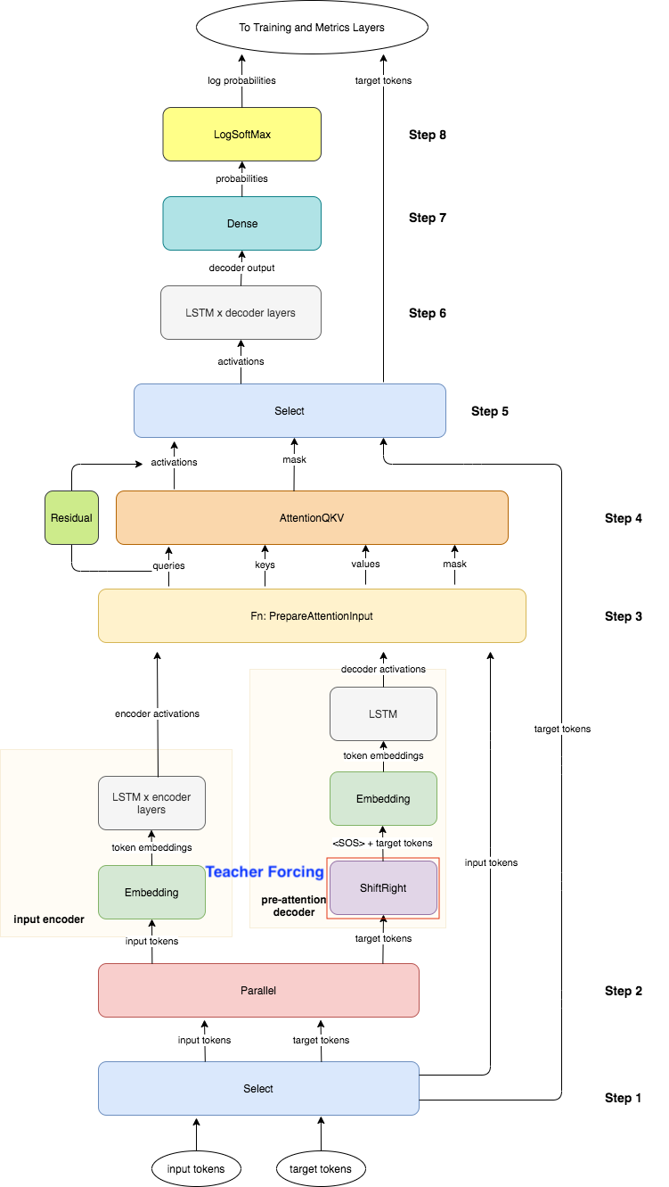
1- Initial select: two copies. Input tokens represented by 0 and the target tokens represented by 1.
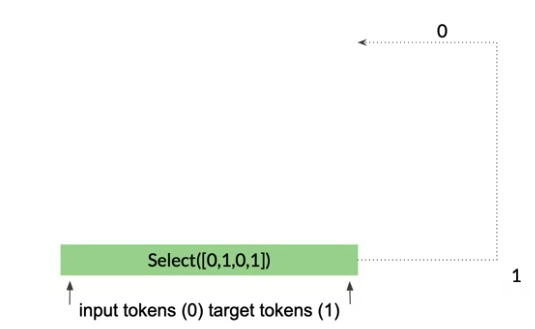
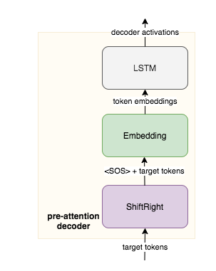
2- One copy of the input fed into as input encoder to be transformed into the key and value vectors. A copy of the target tokens goes into the pre-attention decoder.
- The pre-attention decoder(not decoder produces the decoded outputs) transform the prediction targets into a different vector space called the query vector Q vector, so can calculate the relative weights to give each input word.
ShiftRightin pre-attention decoder shifts the target tokens one place to the right, assign the start of sentence<SOS>to beginning of each sequence, where the teacher forcing takes place.
3- Inputs and targets are converted to embeddings
4- Now have query key and value vectors, you can prepare them for the attention layer:
- Compute \(QK^T\)
- apply a padding mask before computing the softmax.
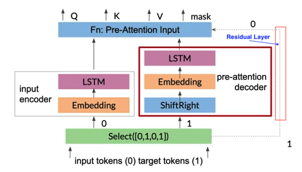
5- Once, have queries, keys, and values, compute attention.
6- Residual block adds the queries generated in the pre-attention decoder to the results of the attention layer. Then attention output its activation along with the mask that was previously created.
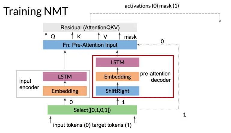
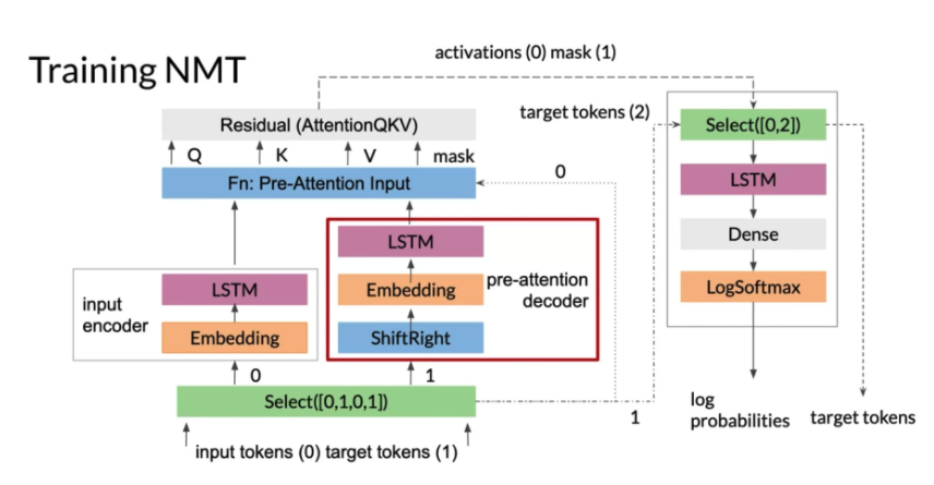
7- Drop the mask(图中标注的mask(1)) before running everything through the decoder, which is what the second Select is doing. Select([0,2]) takes the activations from the attention layer(图中标注的attention(0)), and the second copy of the target tokens(图中标注的target tokens(2). They are true targets which the decoder needs to compare against the predictions.
8- Run through a dense layer with targets vocab size -> gives output.
9- Take the outputs through LogSoftmax, which is what transforms the attention weights to a distribution between zero and one.
10- Match the log probabilites against true target tokens (true target token is outside decoder and pass down to the logsoftmax)
Note: 图中的 Select([0,2]) -> LSTM -> Dense -> LogSoftmax : 是decoder
BLEU Score
BLEU: Bilingual Evaluation Understudy. 缺点: 同义词但n-gram 不一样,low score, 但是good translation. And no consideration of recall
- evaluate the quality of machine-translated text by compaing a candidate texts translation to one or more reference translation.
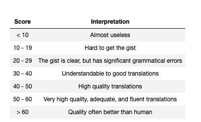
- Usually The closer the BLEU score to one, the better the model. The closer to zero, the worse it is.
- To get the BLEU score, the candidates and the references are usually based on an average of unigram, bigram, trigram or even four-gram.
- Unigrams account for adequacy while longer n-grams account for fluency of the translation.
- Problem
- BLEU doesn’t consider semantic meaning, so does not take into account the order of n-gram
- BLEU doesn’t consider sentence structure.e.g “Ate I was hungry beacause!” 如果reference is “I ate because I was hungry”, will get a perfect BLEU score
Bervity Penalty: The brevity penalty penalizes generated translations that are too short compared to the closest reference length with an exponential decay. The brevity penalty compensates for the fact that the BLEU score has no recall term.(recall: 是不是reference 中的正确都predict了,referenece length > candidate length, no penalty )
\[BP = min \left(1, e^{1- \frac{\text{ref length}}{\text{candidate length}}} \right)\]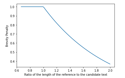
BLEU Score:
\[BLUE = BP \left(\prod_{i=1}^4 precision_i \right)^{\frac{1}{4}}\] \[precision_i = \frac{\sum_{snt \in cand} \sum_{i \in snt} min\left(m_{cand}^i, m_{ref}^i \right)}{w_t^i}\]Where:
- \(m_{cand}^i\) , is the count of i-gram in candidate matching the reference translation.
- \(m_{ref}^i\) , is the count of i-gram in the reference translation.
- \(w_{t}^i\) , is the total number of i-grams in candidate translation.
- \(min\left(m_{cand}^i, m_{ref}^i \right)\) 表示比如 bigram, (I,am) 在candidate中出现5次,但在reference中只出现3次,就取3次
下面图中的score 是乘以100后的结果
ROUGE
F1 score
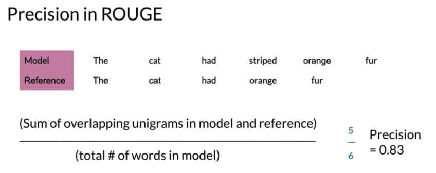
\[score = 2 \frac{ precision * recall}{precision + recall}\]recall-Oriented Understudy for Gisting Evaluation:
- Calculates precision and recall for machine texts by counting the n-gram overlap between the machine texts and a reference text.
- Measures precision and recall between generated text and human-created text where order matters
- precision: How much of model text was relevant
- Recall: How much of the reference text is the system text captures?
- Problem:
- Doesn’t take similar themes or concepts(同义词) into consideration( low ROUGE score doesn’t necessarily mean the the translation is bad) 比如 model predict “I am a fruit-filled pastry” 跟 reference” I am a jelly donut” 意思一样但是score低
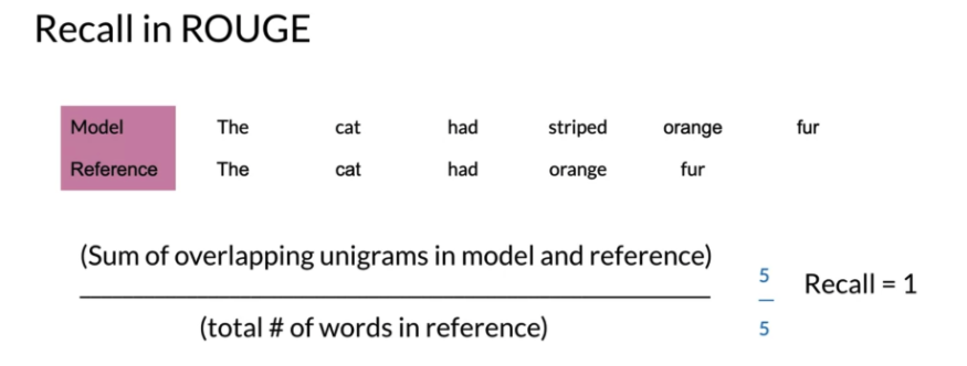
The, cat, had, orange, fur 都appear。 如果model wants a high recall score, can guess hundred of words and have the chance the words in the true reference sentence. Then use precision
def rouge1_similarity(system, reference):
# system (list of int): tokenized version of the system translation

#reference (list of int): tokenized version of the reference translation

    sys_counter = collections.Counter(system)
    ref_counter =  collections.Counter(reference)

    overlap = 0
    for token in sys_counter:
        token_count_sys = sys_counter.get(token,0)
        token_count_ref = ref_counter.get(token,0)
        overlap += min(token_count_sys,token_count_ref)

    precision = overlap/sum(sys_counter.values())
    recall = overlap/sum(ref_counter.values())
    if precision + recall != 0:
        # compute the f1-score

        rouge1_score = 2*(precision*recall)/(precision+recall)
    else:
        rouge1_score = 0
    return rouge1_score
Greedy Decoding
- Select the most probable word at each step(每步选取最大概率的)
- For short sequence, it is fine
- Limitiation: Best word at each time != best for long sequence, 比如model predict 出 I am, am, am, am…
Random Sampling
- Problem of Random Sampling: Often a little too random for accurate translation
- Solution: assign more weight to more probable words, and less weight to less probable words
- Temperature: a parameter allowing for more or less randomness in predictions. measured on scale from 0 to 1, indicating low to high randomness
- Lower temperatue setting = More confident, conservative network. More careful/safe decision for output
- Higher temperatue setting = More excited, random network(and more mistakes)
Below codeis to generate random samplying from log-softmax output. the amount of “noise” added to the input by these random samples is scaled by a temperature setting. If temperature equal to 0 will return the argmax of log_probs(greedy decoding)
def logsoftmax_sample(log_probs, temperature=1.0):
#Returns a sample from a log-softmax output, with temperature.

# log_probs: Logarithms of probabilities (often coming from LogSofmax)

# temperature: For scaling before sampling (1.0 = default, 0.0 = pick argmax)


  # This is equivalent to sampling from a softmax with temperature.

  u = np.random.uniform(low=1e-6, high=1.0 - 1e-6, size=log_probs.shape)
  g = -np.log(-np.log(u))
  return np.argmax(log_probs + g * temperature, axis=-1)
Beam Search
- A broader, more exploratory decoding alternative
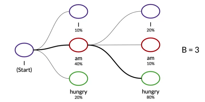
- Istead of offering a best output like greedy decoding, beam seach select multiple options for the best input based on conditional probability
- Beam width B: limit the number of branching paths. Select B number of best alternatives at each time step with the highest probabilities
- A larger beam width -> better model performance but slower decoding speed.
- Problem:
- Since the model learns a distribution, that tends to carry more weight than single tokens
- Can cause translation problems, 比如 in a speech corpus that hasn’t been cleaned. If have filler word “Uhm” which appear as translation with lower probability. at time step, most probable word 是 “Uhm”
Minimum Bayes Risk (MBR)
Alternative of Beam Search
- Generate several random samples using random sampling for outputs
- Compare each sample against all the others and assign a similarity score (such as ROUGE!)
- Select the sample with the highest similarity.
Examples: MBR Sampling, generate the scores for 4 samples: (注是 prediction 和prediction 之间算similarity 不是prediction 和 reference 比)
- Calculate similarity score between sample 1 and sample 2
- Calculate similarity score between sample 1 and sample 3
- Calculate similarity score between sample 1 and sample 4
- Calculate weighted average of first 3 steps (usually a weighted average)
- Repeat until all samples (2,3,4) have overall scores
4.3 Transformer
Transformer
- transformer are based on attention, not require sequential computation per layer, only one step is needed
- Gradient steps from last output to the first input in a transformer is 1 step. For RNN, the number of steps equal to T
- Transformer don’t suffer from vanishing gradient problem which related to the length of sequence
- Transformer differ to Seq2Seq, use Multi-headed attention layer instead of recurrent layer
Tranformer Application
- Text summarization
- Auto-complete(比如打字,comple, 输出complete)
- Named entity recognition(NER)
- Question answering
- Translation
- Chat-bots
- Other NLP tasks e.g. Sentiment Analysis, Market Intelligence, Text Classification, Character Recognition, Spell Checking.
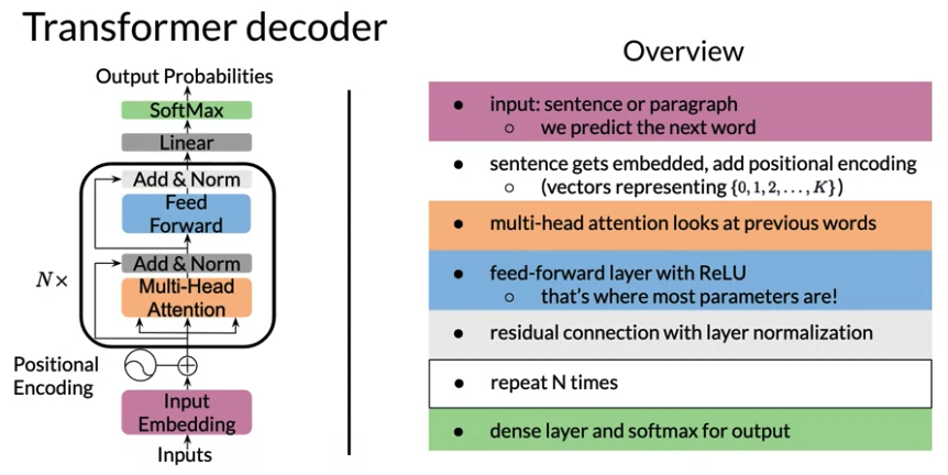
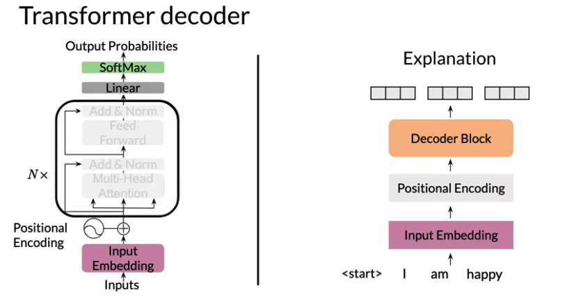
Transformer Decoder (GPT-2)
- Input is tokenized sentence(vector of integer), with shift right layer to add start token
<SOS>which model will used to predict next word - Sentence get embedded with word embeddings
- after embedding, shape is
batch x length x d_model,d_modelusually 512,1024, nowadays up to 10k or more
- after embedding, shape is
- Position Encoding: add embedding the information about position to produce positional input embedding. The information is to learn vector representing
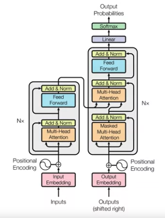
{0,1,2,...k} - Multi-Headed Attention Layer & Feed Forwared: Repeat This Step N times. The transformer repeat \(\geq 100\)steps. (Original paper N=6)
- This model process each word of input sequence from positional input embedding
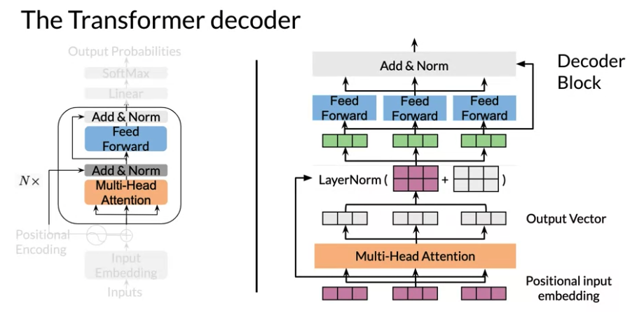
- Multi-Headed Attention: Each layer of attention, there is a resuidual connection, followed by a normalization layer step to speed up training and significantly reduce overall processing time
- Feed-forward layer:
- with ReLU which operates each position independently and each input have shared parameters for efficiency.(对于所有input的的Feedfoward layer share weight 跟RNN一个道理)
- Add drop out as regularization
- After each attention layer and feed-forward layer, put a residual or skip connection. Add inputs of that layer to its output and perform layer normalization
- Finally the encoder layer output is obtained
- Final a dense layer and a softmax layer for output, output
batch x length x # vocabulary - calculate record softmax for cross entropy loss
Transformer Summarizer
Use Transformer model to produce the summary for article.
- Model Input:
article Text <EOS> SUMMARY <EOS> <pad>- input tokenized as a sequence of integers. 0 表示 padding, 1 表示 EOS
- Motivation for weighted Loss: As we know, Transformer only take text as input and predict next word. But we don’t want to penalize to have a huge loss if not predict corrent one
- 0s for all words in article until the first
<EOS>and then 1 for the summary - When there is a little data for summary, it helps to weight article loss with nonzero number say 0.2, 0.5, or even 1 insted of 0. This way, model is able to learn word relationship that are common in the news
- 0s for all words in article until the first
Cost function: cross entropy function that ignores the words from the article to be summarized
\[J = -\frac{1}{m} \sum_j^m \sum_i^K y_j^i log \hat y_j^i\] \[\text{where j: over summary. i: batch elements}\]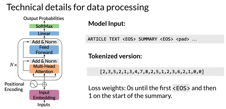
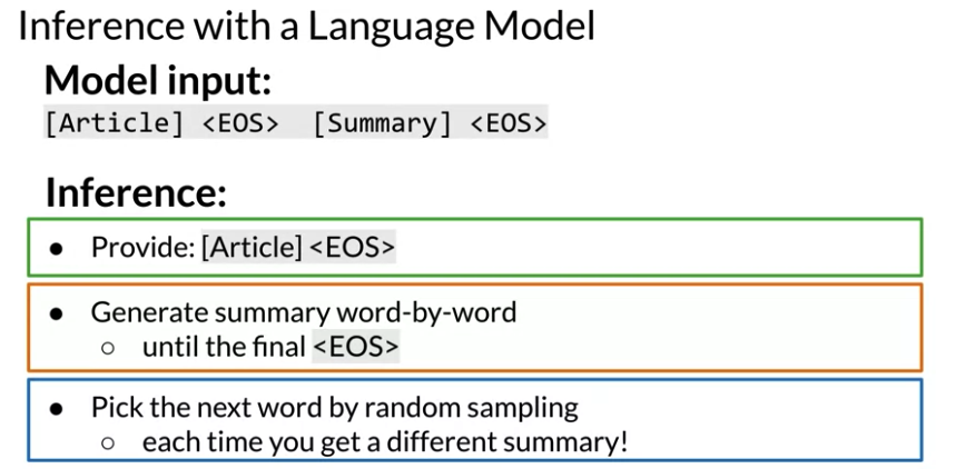
Test or Inference
- input the
article <EOS>token(first word of the summary) to the model - Generate sumary word by random sampling until get
<EOS>.- When run transformer model, sample from probability distrbution over all possible words. So each time get a different summary.
- Model is able to learn word relationship that are common
#article, summary integer vector

joint = np.array(list(article) + [EOS, SEP] + list(summary) + [EOS])
mask = [0] * (len(list(article)) + 2) + [1] * (len(list(summary)) + 1) # Accounting for EOS and SEP
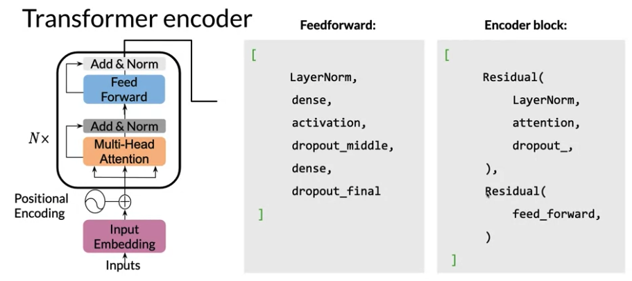
Transformer Decoder Implementation
- In DecoderBlock, position of the LayerNorm in transformer models is still very much a field of research
def PositionalEncoder(vocab_size, d_model, dropout, max_len, mode):
    return [
        tl.Embedding(vocab_size, d_model),
        tl.Dropout(rate=dropout, mode=mode),
        tl.PositionalEncoding(max_len=max_len, mode=mode)]

def FeedForward(d_model, d_ff, dropout, mode, ff_activation):
    #d_ff (int): depth of feed-forward layer.(dimension of Dense output)

    return [
        tl.LayerNorm(),
        tl.Dense(d_ff),
        # Add activation function passed in as a parameter

        ff_activation(),  # Generally ReLU

        tl.Dropout(rate=dropout, mode=mode),
        tl.Dense(d_model),
        tl.Dropout(rate=dropout, mode=mode)
    ]

def DecoderBlock(d_model, d_ff, n_heads,
                 dropout, mode, ff_activation):

    return [
      tl.Residual(
          tl.LayerNorm(),
          tl.CausalAttention(d_model, n_heads=n_heads, dropout=dropout, mode=mode)
        ), #Query + Output(LayerNorm(), CausalAttention)

          # Instead of Query + Output(LayerNorm()) + Query + CausalAttention

      tl.Residual(
          # We don't need to normalize the layer inputs here. The feed-forward block takes care of that for us.

          FeedForward(d_model, d_ff, dropout, mode, ff_activation)
        ), #Query + Output(FeedForward)

      ]

def TransformerLM(vocab_size=33300,
                  d_model=512,
                  d_ff=2048,
                  n_layers=6,
                  n_heads=8,
                  dropout=0.1,
                  max_len=4096,
                  mode='train',
                  ff_activation=tl.Relu):

    # Create stack (list) of decoder blocks with n_layers with necessary parameters

    decoder_blocks = [
        DecoderBlock(d_model, d_ff, n_heads, dropout, mode, ff_activation) for _ in range(n_layers)]

    return tl.Serial(
        # Use teacher forcing (feed output of previous step to current step)

        tl.ShiftRight(mode=mode),
        # Add embedding inputs and positional encoder

        PositionalEncoder(vocab_size, d_model, dropout, max_len, mode),

        decoder_blocks,
        tl.LayerNorm(),
        # Add dense layer of vocab_size (since need to select a word to translate to)

        #tl.Mean(axis=1), can add a mean layer

        # (a.k.a., logits layer. Note: activation already set by ff_activation)

        tl.Dense(vocab_size),
        # Get probabilities with Logsoftmax

        tl.LogSoftmax()
    )
4.4 Question Answering
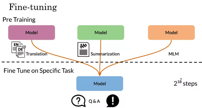
Transfer Learning
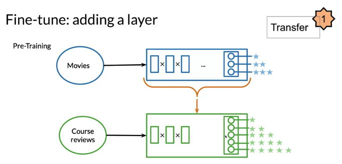
Goal of Transfer Learning: e.g. use pretrain model (movie review) on course review.
- Reduce training time, faster convergence
- Improve predictions
- require a small datasets, because model learn a lot from other tasks
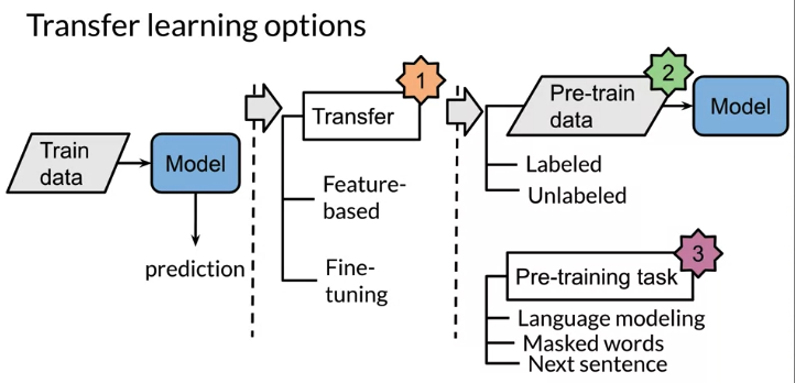
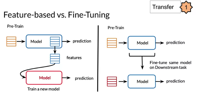
Two methods in Transfer learning
- Feature based method, use pre-trained word embeding(use pretrain CBOW) as feature to feed in your own model
- Fune tuning method,
- take a exisitng weights(e.g. from word embeddings) as initialized weights and fine tune them on new task
- Also can add a new layer and only fine tune new layer keep other layer frozen 比如 movie review predict 3 ratings, course review provide 5 ratings, add a new layer to match new dimension(5)
Generaly, a bigger dataset -> a larger model -> better performance.
The amount of unlabeled data is larger than labeled data.
- Use unlabeled data for pre-training. 比如CBOW, mask random word to learn the word from the context(self-supervised learning)
- In downstream tasks, Use model wweights from step 1 to predict labeled data
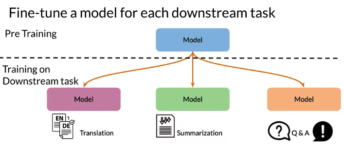
Have a initial weight and fine tune on each different downstream task. Then use this model to translate English to German, summarization, or do question answering.
The model that is trained bidirectionally may have a deeper sense of context and language flow than unidirectional models.
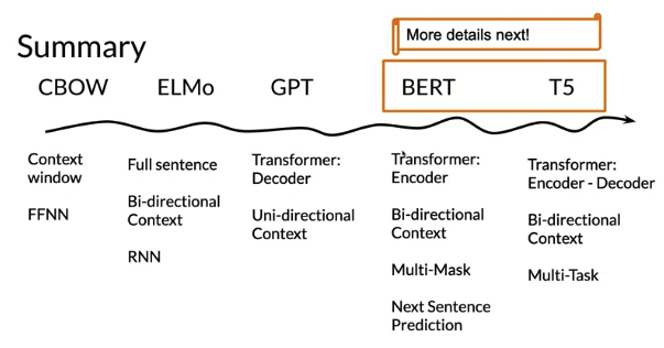
ELMo, GPT, BERT, T5
- ELMo: CBOW using C as windows size, ELMo use full context using RNN (Bi-directional LSTM) to predict the center word. Also suffer long-term dependency problem
- GPT(Decoder): uni-directional(only look at previous attention(No peeking itself, not look at current word or future word). only has transformer Eecoder not encoder. self-attention(Each word can peek at itself), but in GPT,
- BERT: bi-drectional. Only has transformer Encoder no Decoder.
- BERT Pre-training Tasks:
- Multi-Mask Langauage modelling. 比如 mask several words in sentence to predict. E.g. “on the _ side _ history”, and model should learn to predict “right” “of”
- Next Sentence Predict: Not only predict word, also learn to predict next sentence. Given Sentence A, 然后给几个选项, predict which one sentence B
- BERT Pre-training Tasks:
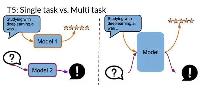
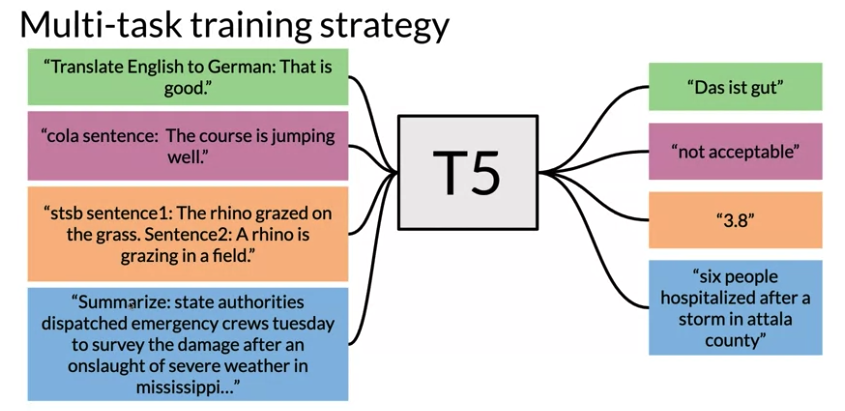
- T5 using Encoder & Decoder: used in Multi-task learning
- To do multi-tasking, append a tag at the beginning of sentence, such as “classify”, “Summarize”, “Question”

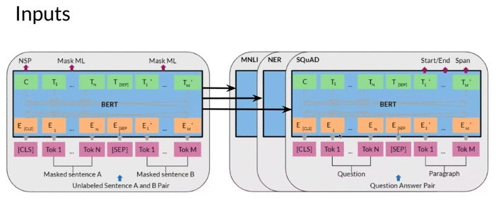
BERT
BERT: Bidirectional Encoder Representation from Transformer
- Start with Embedding and positional embeddings, and get \(E_1, E_2 ... E_N\)
- Go to Transformer block(图中的蓝色圈)
- Get \(T_1, T_2 ... T_N\)
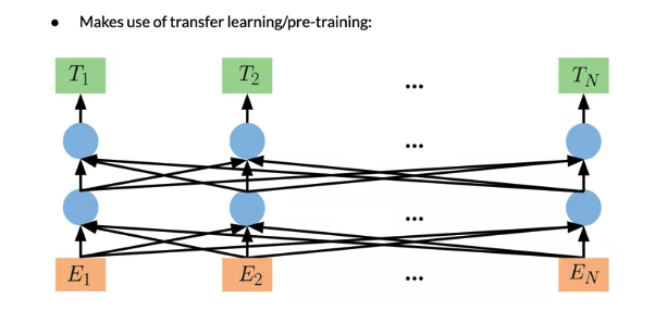
- Pretraining: use unlabelled data over different pretraining tasks
- Mask language modelling(MLM) :
- Before feeding word sequences to BERT model, randomly picked 15% of the tokens in the input for prediction. These tokens are pre-processed as follows — 80% are replaced with a
[MASK]token, 10% with a random word, and 10% use the original word. More explanations for this kind of masking-Appdix A - Add a Dense layer(multiply output vector by the embedding matrix) after encoder outputs \(T_i\) then transform them into vocabulary dimension and add softmax
- Next sentence prediction is also used when pre-training: Given two sentences, if true means two sentence follow one another.
- Before feeding word sequences to BERT model, randomly picked 15% of the tokens in the input for prediction. These tokens are pre-processed as follows — 80% are replaced with a
- Mask language modelling(MLM) :
- Fine-tuning: initialized with pre-trained parameters and all of pararmeters are fine-tuned using labeled data from downstream task
Famous model is BERT_base, has: (New model come out now has more parameters)
- 12 layers(12 transformer blocks)
- 12 attentions heads
- 110 million parameter
Objective
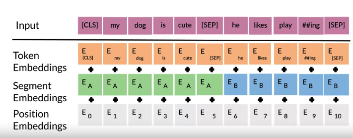
- start with positional embedding which indicate the position in the sentence of the word
- Then have segment embeddings: 表示if it is sentence A or sentence B (because BERT aslo use next sentence predictions)
- Then have token embedding/input embedding, also have
CLStoken 表示beginning of sentence, a special classification symbol added in front of every input 和SEPtoken 表示 end of sentence. - Take the sum of those embedding to get a new input \(Tok1, \cdots Tok N\) and \(Tok1, \cdots Tok M\)
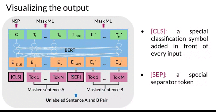
5. Convert the new input using embedding and pass to Transformer block
- new input unlabeled sentence A/B in the image will depend on what you are trying to predict, it could range from question answering to sentiment (in which case second sentence just empty)
6. In the end get \(T_1 , \cdots T_N\) and \(T_1' , \cdots T_M'\) prediction for masked word
- \(T_i\) embedding are used to predict masked word using softmax.
- 绿色的C token in the image above could be used for classification purposes.
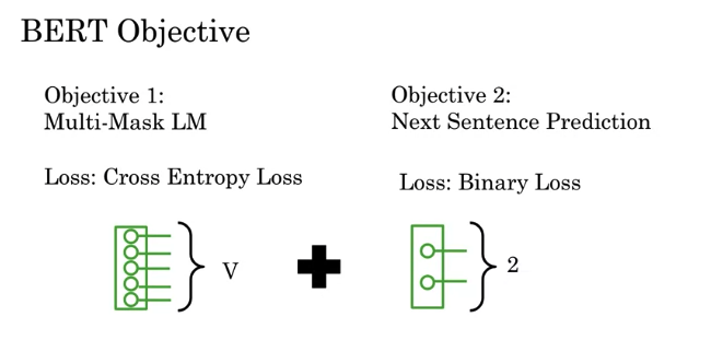
BERT Objective: Cross Entropy Loss + Binary Loss
- Objective 1: For Multi-Mask Language Model, use Cross Entropy Loss to predict the word being masked
- Objective 2: Add Binary loss for Next Sentence Prediction
Fine Tuning
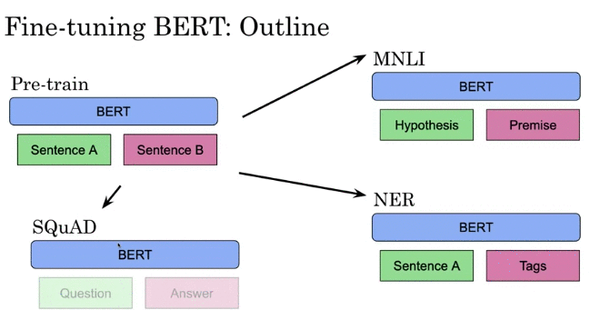
- During Pre-train of BERT, have sentence A and B and use next sentence prediction
- Then fine tune on different tasks such as Hypothesis Premise or NER task, Questions Answering
- feed Hypothesis at Sentence A input Position, feed Premise at Sentence B input position
- NER task: feed Sentence A at Sentence A input Position, feed Tags at Sentence B input position
- Question Answering: feed Questions at Sentence A input Position, feed Answer at Sentence B input position
Some other downstream task that can use Pre-train BERT model
T5
T5 transformer known as Text to Text transformer. T5 model use similar training strategy as BERT. It make use of transfer learning and mask langauage modeling. T5 also use Transformer when training. Can used for
- Classification
- Question Answering
- Machine Translation
- Summarization
- Sentiment
Pre-training:(same as BERT) mask certain words. The bracket use in increment order. 下面例子用了 <X> <Y> <Z> 那么接下来的 mask 用 <A> <B>
e.g. Original Text: Thank you for inviting me to your party last week
- Inputs:
Thank you <X> me to your party <Y> week - Target:
<X> for inviting <Y> last <Z>
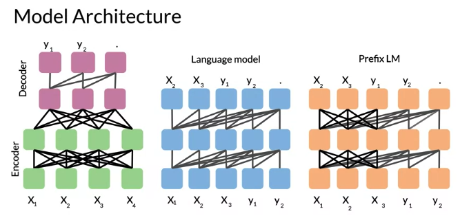
Model Architecture: Use Encoder/decoder stack, total 12 transformer blocks each, 220 million parameters
- Basic Encoder-Decoder Representation: Fully visible attention in Encoder and causal attention in Decoder
- Language model: single transformer layer stack which are fed the concatenation of inputs and target, use causal attention
- Prefix Language model: fully visible masking over inputs(for X) and causal masking(for Y)
Multi-Task Training Strategy
Add task at the prefix of input sentence. T5 framework provides a consistent training objective both for pre-training and fine-tuning. Specifically, the model is trained with a maximum likelihood objective (using “teacher forcing” ) regardless of the task.
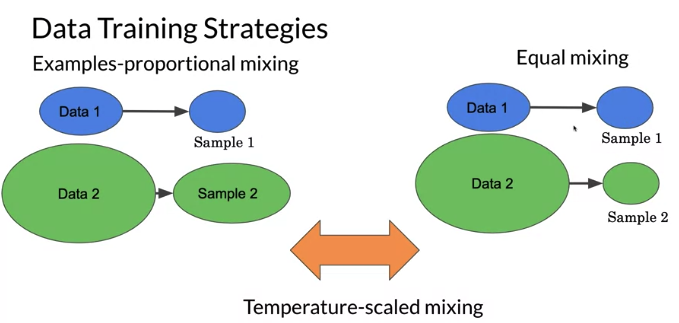
- Examples-proportional mixing: 每个dataset 不管多大多小,都take 10%. sample in proportion to the size of each task’s dataset
- Equal mixing: regardless size of data, sample examples from each task with equal probability. Specifically, each example in each batch is sampled uniformly at random from one of the datasets you train on.
- Temperature scaled mixing: play the paratmeters to get something between Examples-proportional mixing and Example mixing,
- To implement temperature scaling with temperature T, we raise each task’s mixing rate
rmto the power of1⁄Tand renormalize the rates so that they sum to 1. When T = 1, this approach is equivalent to examples-proportional mixing and as T increases the proportions become closer to equal mixing
- To implement temperature scaling with temperature T, we raise each task’s mixing rate
Graudal Unfreezing: freeze one layer at a time. 比如下图 freeze last layer, fine-tuned using that keep other fixed. Then freeze 倒数第二个… gradual freezing each layer
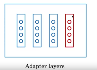
Adapter layers:
- add existing neural network or a neural network to each feed forward and each block of the transformer. Then these new feed forward networks designed that output dimension match input, allows them to be inserted without having ay structural change.
- When fine-tuning, only new adapter layers and layer normalization are updated
A single model can simultaneously perform many tasks at once. Model most of parameters are shared across all of the tasks. Might train a single model on many tasks, but when reporting performance, can select different checkpoints for each task. Do the train at 2^18 steps
GLUE Benchmark
GLUE: General Language Understanding Evaluation
- A collection used to train, evaluate, analyze natural language understanding systems
- has a lot of datasets. Each Dataset with different genres, and of different size and difficulties. 比如some are for coreference resolution, other used for simple sentiment analysis
- Used with a leaderboard: people can use dataset, see how well models perform compared to others
Tasks Evaluated on
- Sentence grammatical or not? Sentence make sense or not?
- Sentiment
- Paraphrase
- Similarity
- Questions duplicates
- Answerable: whether question can be answered or not?
- Contradiction
- Entailment
- Winograd: try to identify whether a pronoun refer to a certain noun or another noun.
Evaluation / Application
- researchers use GLUE as a benchmark
- Model agnostic, doesn’t matter which model you used
- allow use of transfer learning because have access to several datasets
Question Answering
4.5 Chatbot
Long Text Sequence deep learning model Chanllenges due to size in training.
- Writing Books: become more difficult to recognize a book written by human or AI
- Chatbots: become more difficult to recognize conversation you have real or computer
AI Storytelling: Dragon model for Dungeon is based on GPT-3. It generates an interactive story based on all previous turns as inputs. That makes for a task that uses very long sequences.
Process long text sequence is core of chatbot. Chatbot use all previous pieces of converversation as inputs for next reply. This make a big context windows
- Context-based question: need both a question and relevant text from where to retrieve answer
- Close loop question. no need extra text with a question or prompt from human. All knowledge is stored in weights of model during training
Transformer Issues
- Attention on sequence of Length L takes \(L^2\) time and memory.
- 比如attention on two sentences of length L, need to compare each word in first sentence to each word in second sentence. 比如 L = 10000, \(L^2\) = 100 M, 如果每秒process 10M, take 10 sec to compute - N Attention layers take N times as much memory. e.g. GPT-3 has 96 layers and new models will have more. Even modern GPU can struggle this dimensionality
- Attention Complexity: Attention is \(softmax\left( QK^T \right)V\),
- assume Queries,Keys,Values are all size L (length) by \(d_{model}\) (depths of attention), Then \(QK^T\) size is L by L.
- For long sequence, usually don’t need consider all L positions, instead focus on area of interest. 比如translate a long text from English to German, don’t need to consider every word at once. Instead focus on single word being translated and those immediately around it by using attention.
- The more layer model has, the more memory need.
- This is because need to store forward pass acivations for backprop. Can overcome this memory requirements by recomputing activations, but it needs to be done efficiently to minimize taking too much extra time. 比如GPT-3 has 96 layers 会take a very long time to recompute activations, and new model will continue to get bigger.
- Compute vs memory tradeoff
LSH Attention
Solve Dot product Attention Complexity
e.g. 比如下图,can see what attention is doing, 比如word it, attention focus on certain words to determine if it refers to the streets or to be animal. it 只能refer to noun not other words 可以ignore other word. A pronoun(it) is a word that substitutes for a noun. That’s why only want to look up nearest neighbor to speed up attention
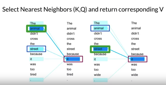
Nearest Neighbors: Compute the nearest neighbors to q among vectors {\(k_1, ...k_n\)}
- Attention computes \(d\left(q,k_i \right)\) for i from 1 to n which can be slow
- Faster approximate uses locality sensitive hashing(LSH)
- Locality sensitive: if q is close to \(k_i\) -> hash(q) == hash(\(k_i\))
- When choose hash, want to make buckets roughly the same size
- only run attention on keys that are in the same hash buckets as the query (就像上边 noun 和 pronoun的例子)
- Achieve by randomly cutting space: hash(x) = sign(xR) where R: [d,n_hash_bins]. R is random, size 是 d(dimension) 乘以 number of hash bins. Sign tell which side of the plane hash will be on. The process is repeated depending # number of hashes
Standard Attenion:
\[A\left(Q,K,V\right) = softmax\left(Qk^T\right)V\]LSH Attention: Note LSH is a probabilistic, not deterministic model 因为inherent randomness within LSH algorithm. Meaning hash can change along with buckets that vector map to
- First hash Q and K
- perform standard attention but within same-hash bins. This reduces the search space for each K to the same LSH bucket as Q. Can repeat this process multiple time to increase the probability of finding Q and K in the same bin. 可以done efficiently by parallel computing
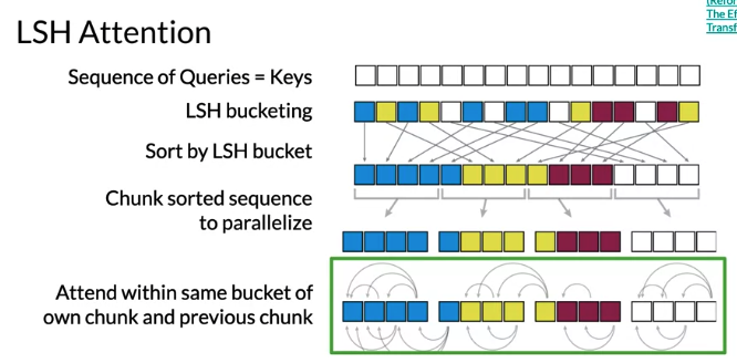
Integrate LSH to attention layer:
- modify model so outputs a single vector at each position which serves both as a query and a key. Called QK attention and performs just as regular attention
- map each vector to a bucket with LSH.
- Sort vectors by LSH bucket
- Do attention only in each bucket. Use batch(parallel) computation 1. split sorted sequence into fixed size chunks which allow parallel computation
- Let each chunk attend within itself and adjacent chunks(比如图中 blue 相互计算, 黄色相互计算, 红色相互计算) 因为一个hash bucket may split more than one chunk
Reversible Layers:
Memory grow linearly with the number of layers
比如 want to run transformer on entire text of book.
- Maybe have 1 million token to process. each token has feature size 512 (比如embedding) -> model input就有 2 GB, 在16GB的GPU, 相当于1/8. Not even touch layer yet.
- Transformer has Attention layer and Feedforward layer. 比如model 有 12个attention, 12个feedforward. 每个layer input 和 output 也是2GB, do backprop, forward path需要store intermediate quantities in meomory. 比如只save activation from boundaries between each layers 不保存individual layer就已经50GB (24 x 2GB + input 2 GB 任何device 都不能fit) 而modern Transformer much deeper than 12 layers
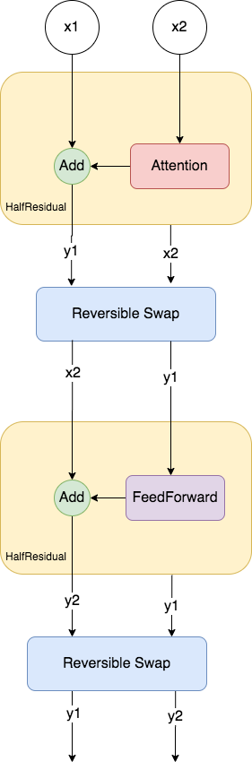
Transformer network precedes repeating by adding residuals to hidden state. To run reverse, can substract residuals in oppsite order, start with outputs of model. In order to save memory, Instead of store residuals, able to recompute quickly instead where residual connection come in. Key idea is start with two copies of model inputs, then each layer only update one. The activation don’t update is the one to compute residuals.
Reversible Residual Blocks: can work for Backprop without saving huge memory for activations in the forward pass
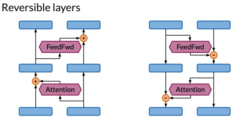
- start with two copies of model inputs, then each layer only update one of two. The activation don’t update is the one to compute residuals.
- Activation in the model is twice as big, don’t worry about catching backward pass
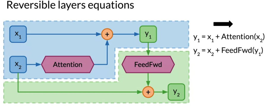
- 下面例子,
- calculate \(y_1 = x_1 + Attention \left( x_2 \right)\)
- calculate \(y_2 = x_2 + Attention \left( y_1 \right)\). \(y_2\) is depended on \(y_1\)
- Foward layer for residual block: combine regular Transformer standard attention and feed forward residual layers to a single reversible residual block. Only save \(y_1, y_2\) of output layer in the memory instead of activiation for every individual layer
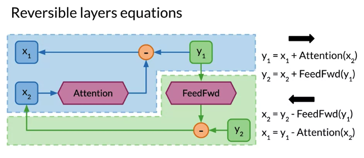
- Backward pass:
- calculate \(x_2\) before \(x_1\), because \(x_1\) has a dpendency on \(x_2\) you just calculate
Note: After each attention layer/Feed Forward layer, swap the elements to take into account the stack semantics in Trax
Roughly the same BLEU scores for regular and reversible transformers on machine translation and language modeling produce similar results. Reversible layer is a general techniques that can be applied anywhere in a transformer model.
Reformer
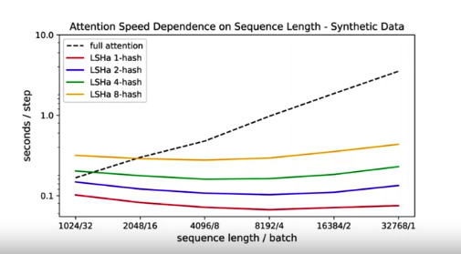
Reformer is a transformer model designed to be memory efficient so it can handle very large context windows of up to 1 million words on a single 16 GB GPU.
- use LSH Attention: reduce complexity of attending over long sequences
- use Reversible Residual Layers: more efficienctly use memory available
下面图from Reformer paper, highlight standard attention takes longer as sequence length increases. However, LSH attention takes roughly the same amount of time as sequence increase. The only difference is number of hashes. More hashes take slightly longer than fewer hashes, regardless of seqeunce sequence,
Resource
The Real Meaning of Ich Bin ein Berliner: Word Alignment: 比如德语 Berliner 可以指柏林人,也可以值一种donut 甜甜圈. 比如下面English word 多于German word.
Jukebox - A neural network that generates music!
GPT-3 Can also help with auto-programming!
Reformer: The Efficient Transformer (Kitaev et al, 2020)
Attention Is All You Need (Vaswani et al, 2017)
Deep contextualized word representations (Peters et al, 2018)
The Illustrated Transformer (Alammar, 2018)
The Illustrated GPT-2 (Visualizing Transformer Language Models) (Alammar, 2019)
How GPT3 Works - Visualizations and Animations (Alammar, 2020)